Crystal Graph Neural Networks

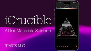
	[Demo Video] The iOS app, iCrucible, uses the CGNN technology to discover new compounds.

This repository contains the original implementation of the CGNN architectures described in the paper "Crystal Graph Neural Networks for Data Mining in Materials Science".

Logo

Gilmer, et al. investigated various graph neural networks for predicting molecular properties, and proposed the neural message passing framework that unifies them. Xie, et al. studied graph neural networks to predict bulk properties of crystalline materials, and used a multi-graph named a crystal graph. Schütt, et al. proposed a deep learning architecture with an implicit graph neural network not only to predict material properties, but also to perform molecular dynamics simulations. These studies use bond distances as features for machine learning. In contrast, the CGNN architectures use no bond distances to predict bulk properties at equilibrium states of crystalline materials at 0 K and 0 Pa, such as the formation energy, the unit cell volume, the band gap, and the total magnetization.

Note that the crystal graph represents only a repeating unit of a periodic graph or a crystal net in crystallography.

Requirements

Python 3.7
PyTorch 1.1+
Pandas
Matplotlib (necessary for plotting scripts)

Installation

git clone https://github.com/Tony-Y/cgnn.git
CGNN_HOME=`pwd`/cgnn

Usage

The user guide in this GitHub Pages site provides the complete explanation of the CGNN architectures, and the description of program options. Usage examples are contained in the directory cgnn/examples.

Dataset Files

The CGNN code needs the following files:

targets.csv consists of all target values.
graph_data.npz consists of all node and neighbor lists of graphs.
config.json defines node vectors.
split.json defines data splitting (train/val/test).

Target Values

targets.csv must have a header row consisting name and target names such as formation_energy_per_atom, volume_deviation, band_gap, and magnetization_per_atom. The name column must store identifiers like an ID number or string that is unique to each example in the dataset. The target columns must store numerical values excluding NaN and None.

Crystal Graphs

You can create a graph data file (graph_data.npz) as follows:

graphs = dict()
for name, structure in dataset:
    nodes = ... # A species-index list
    neighbors = ... # A list of neighbor lists
    graphs[name] = (nodes, neighbors)
np.savez_compressed('graph_data.npz', graph_dict=graphs)

where name is the same identifier as in targets.csv for each example.

tools/mp_graph.py creates graph data from structures given in the Materials Project structure format. This tool is used when the OQMD dataset is compiled.

Node Vectors

You can create a configuration file (config.json) using the one-hot encoding as follows:

n_species = ... # The number of node species
config = dict()
config["node_vectors"] = np.eye(n_species,n_species).tolist()
with open("config.json", 'w') as f:
    json.dump(config, f)

Data Splitting

You can create a data-splitting file (split.json) as follows:

split = dict()
split["train"] = ... # The index list for the training set
split["val"] = ... # The index list for the validation set
split["test"] = ... # The index list for the testing set
with open("split.json", 'w') as f:
    json.dump(split, f)

where the index, which must be a non-negative integer, is a row label of the data frame that the CSV file targets.csv is read into.

Training

A training script example:

NodeFeatures=... # The size of a node vector
DATASET=${CGNN_HOME}/YourDataset
python ${CGNN_HOME}/src/cgnn.py \
  --num_epochs 100 \
  --batch_size 512 \
  --lr 0.001 \
  --n_node_feat ${NodeFeatures} \
  --n_hidden_feat 64 \
  --n_graph_feat 128 \
  --n_conv 3 \
  --n_fc 2 \
  --dataset_path ${DATASET} \
  --split_file ${DATASET}/split.json \
  --target_name formation_energy_per_atom \
  --milestones 80 \
  --gamma 0.1 \

You can see the training history using tools/plot_history.py that plots the root mean squared errors (RMSEs) and the mean absolute errors (MAEs) for the training and validation sets. The values of the loss (the mean squared error, MSE) and the MAE are written to history.csv for every epoch.

python ${CGNN_HOME}/tools/plot_history.py

After the end of the training, predictions for the testing set are written to test_predictions.csv. You can see the predictions compared to the target values using tools/plot_test.py.

python ${CGNN_HOME}/tools/plot_test.py

Prediction

The prediction for new data is conducted using the testing-only mode of the program. You first prepare a new dataset with a testing set including all examples to be predicted. The prediction configuration must have all the same parameters as the training configuration except for the total number of epochs, which must be zero for testing only. In addition, you must specify the model to be loaded using --load_model YourModel.

DATASET=${CGNN_HOME}/NewDataset
python ${CGNN_HOME}/src/cgnn.py \
  --num_epochs 0 \
  --batch_size 512 \
  --lr 0.001 \
  --n_node_feat ${NodeFeatures} \
  --n_hidden_feat 64 \
  --n_graph_feat 128 \
  --n_conv 3 \
  --n_fc 2 \
  --dataset_path ${DATASET} \
  --split_file ${DATASET}/split.json \
  --target_name formation_energy_per_atom \
  --milestones 80 \
  --gamma 0.1 \
  --load_model ${MODEL} \

The Open Quantum Materials Database

The OQMD v1.2 contains 563k entries, and is available from the OQMD site. The detail setup of the database is described in the README in the directory cgnn/OQMD. Alternatively, you may use the OQMD v1.2 dataset available at this link. There is a data loading tutorial.

Note that there is an abnormal entry in this dataset. The information is available at this page.

Citation

When you mention this work, please cite the CGNN paper:

@techreport{yamamoto2019cgnn,
  Author = {Takenori Yamamoto},
  Title = {Crystal Graph Neural Networks for Data Mining in Materials Science},
  Address = {Yokohama, Japan},
  Institution = {Research Institute for Mathematical and Computational Sciences, LLC},
  Year = {2019},
  Note = {https://github.com/Tony-Y/cgnn}
}

References

Justin Gilmer, et al., "Neural Message Passing for Quantum Chemistry", Proceedings of the 34th International Conference on Machine Learning (2017) arXiv GitHub
Tian Xie, et al., "Crystal Graph Convolutional Neural Networks for an Accurate and Interpretable Prediction of Material Properties", Phys. Rev. Lett. 120, 145301 (2018) DOI arXiv GitHub
Kristof T. Schütt, et al., "SchNet - a deep learning architecture for molecules and materials", J. Chem. Phys. 148, 241722 (2018) DOI arXiv GitHub

License

Apache License 2.0

Tony-Y / cgnn

readme