![]()
Hotspot
Hotspot is a tool for identifying informative genes (and gene modules) in a single-cell dataset.
Importantly 'informative' is decided based on how well a gene's variation agrees with some cell metric - some similarity mapping between cells.
Genes which are informative are those whose expression varies in similar way among cells which are nearby in the given metric.
The choice of metric allows you to evaluate different types of gene modules:
- Spatial: For spatial single-cell datasets, you can define cell similarity by proximity in physical, 2D/3D space. When set up this way, Hotspot can be used to identify spatially-varying genes.
- Lineage: For single-cell datasets with a lineage tracing system, you can infer a cell developmental lineage and use that as the cell metric. Then Hotspot can be used to identify heritable patterns of gene expression.
- Transcriptional: The result of a dimensionality reduction procedure can be used create the similarity metric. With this configuration, Hotspot identifies gene modules with local correlation. This can be particularly useful for interpreting axes of variation in non-linear dimensionality reduction procedures where the mapping between components and genes is not straightforward to evaluate.
Examples
Other Links
Installation
Hotspot is installed directly from PyPI using the following command:
pip install hotspotscHotspot can be imported as
import hotspotStarting with v1.0, Hotspot uses the AnnData data object. If you'd like to use the old version of Hotspot then:
pip install hotspotsc==0.9.1The old documentation for that version can be found here, but installation will still be pip install hotspotsc==0.9.1.
The old initialization for v0.9.1 has now moved to hotspot.Hotspot.legacy_init, see the docs for usage.
Usage
The following steps are used when analyzing data in Hotspot:
- Create the Hotspot object
- Compute the KNN graph
- Find informative genes (by gene autocorrelation)
- Evaluate pair-wise gene associations (gene local correlations)
- Group genes into modules
- Compute summary per-cell module scores
Here we describe each step in order:
Create the Hotspot object
To start an analysis, first create the hotspot object When creating the object, you need to specify:
- The gene counts matrix
- Which background model of gene expression to use
- The metric space to use to evaluate cell-similarity
- The per-cell scaling factor
- By default, number of umi per cell is used
For example:
import hotspot
hs = hotspot.Hotspot(
    adata,
    layer_key="counts",
    model='danb',
    latent_obsm_key="X_pca",
    umi_counts_obs_key="total_counts"
)
In the example above:
adatais a AnnData object of cells by geneslayer_keyis the layer ofadatacontaining count informationmodel'danb' selects the umi-adjusted negative binomial modellatent_obsm_keyis the.obsmkey ofadatacontaining Cells x Components matrix (the PCA-reduced space)umi_counts_obs_keyis the.obskey ofadatawith the UMI count for each cell
Alternative choices for 'model'
The model is used to fit per-cell expectations for each gene assuming no correlations. This is used as the null model when evaluating autocorrelation and gene-gene local correlations. The choices are:
- danb: 'Depth-adjusted negative binomial' (aka NBDisp model) from M3Drop
- bernoulli: Here only the detection probability for each gene is estimated. Logistic regression on gene bins is used to evaluate this per-gene and per-cell as a function of the cells
umi_countvalue. - normal: Here expression values are assumed to be normally-distributed and scaled by the values in
umi_count. - none: With this option, the values are assumed to be pre-standardized
Choosing different metrics
Above we used latent_obsm_key as the input option. This assumes that cells are in an N-dimensional space and similarity between cells is evaluated by computing euclidean distances in this space. Either the results of a dimensionality reduction or modeling procedure can be input here, or when working with spatial data, the per-cell coordinates.
Alternately, instead of latent_obsm_key, you can specify either tree or distances_obsp_key.
tree is used for a developmental lineage. In this form, tree should be an ete3.TreeNode object representing the root of a Tree with each cell as its leaves. This could be constructed programmatically (see ete3's documentation for details) or if your lineage is stored in a Newick file format, you can load it into an ete3.TreeNode object by running ete3.Tree('my_newick.txt'). Note: leaf nodes in the tree must have names that match the column labels in the counts input (e.g., cell barcodes).
distances_obsp_key is used to specify cell-cell distances directly. The value entered should be a Cells x Cells matrix in adata.obsp.
Compute the KNN graph
The K-nearest-neighbors graph is computed by running:
hs.create_knn_graph(weighted_graph=False, n_neighbors=30)Input options:
weighted_graph: bool, whether or not the graph has weights (scaled by cell-cell distances) or is binaryn_neighbors: the number of neighbors per cell to use. Larger neighborhood sizes can result in more robust detection of correlations and autocorrelations at a cost of missing more fine-grained, smaller-scale patterns and increasing run-timeneighborhood_factor: float, used whenweighted_graph=True. Weights decay proportionally toexp(-distance^2/distance_N^2)wheredistance_Nis the distance to then_neighbors/neighborhood_factorth neighbor.
Generally, the above defaults should be fine in most cases.
Find informative genes (by gene autocorrelation)
To compute per-gene autocorrelations, run:
hs_results = hs.compute_autocorrelations()An optional argument, jobs can be specified to invoke parallel jobs for a speedup on multi-core machines.
The output is a pandas DataFrame (and is also saved in hs.results):
| Gene | C | Z | Pval | FDR |
|---|---|---|---|---|
| ENSG00000139644 | 0.069 | 10.527 | 3.21e-26 | 7.45e-25 |
| ENSG00000179218 | 0.071 | 10.521 | 3.43e-26 | 7.93e-25 |
| ENSG00000196139 | 0.081 | 10.517 | 3.59e-26 | 8.28e-25 |
| ENSG00000119801 | 0.062 | 10.515 | 3.68e-26 | 8.48e-25 |
| ENSG00000233355 | 0.058 | 10.503 | 4.15e-26 | 9.55e-25 |
| ... | ... | ... | ... | ... |
Columns are:
C: Scaled -1:1 autocorrelation coeficientsZ: Z-score for autocorrelationPval: P-values computed from Z-scoresFDR: Q-values using the Benjamini-Hochberg procedure
Evaluate pair-wise gene associations (gene local correlations)
To group genes into modules, we need to first evaluate their pair-wise local correlations
Better than regular correlations, these 'local' correlations also take into accounts associations where one gene, X, is expression 'near' another gene Y in the map. This can better resolve correlations between sparsely detected genes.
hs_genes = hs_results.loc[hs_results.FDR < 0.05].index # Select genes

local_correlations = hs.compute_local_correlations(hs_genes, jobs=4) # jobs for parallelization
Here we run only on a subset of genes as evaluating all pair-wise correlations is very expensive computationally. The autocorrelation ordering gives us a natural method to select the informative genes for this purpose.
The output is a genes x genes pandas DataFrame of Z-scores for the local correlation values between genes. The output is also stored in hs.local_correlation_z.
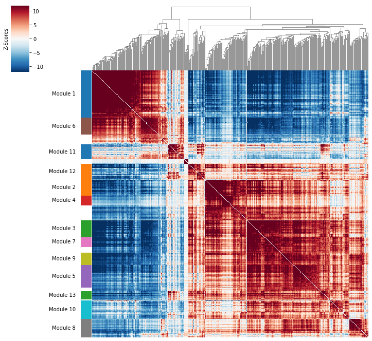
Group genes into modules
Now that pair-wise local correlations are calculated, we can group genes into modules.
To do this, a convenience method is included create_modules which performs
agglomerative clustering.
modules = hs.create_modules(
    min_gene_threshold=30, core_only=True, fdr_threshold=0.05
)
A note on the arguments - agglomerative clustering proceeds by joining together genes with the highest pair-wise Z-score with the following caveats:
- If the FDR-adjusted p-value of the correlation between two branches exceeds
fdr_threshold, then the branches are not merged. - If two branches are two be merged and they are both have at least
min_gene_thresholdgenes, then the branches are not merged. Further genes that would join to the resulting merged module smaller average correlations between genes, i.e. the least-dense module (ifcore_only=False)
This method was used to preserved substructure (nested modules) while still giving the analyst
some control. However, since there are a lot of ways to do hierarchical clustering, you can also
manually cluster using the gene-distances in hs.local_correlation_z
The output is a pandas Series that maps gene to module number. Unassigned genes are indicated with a module number of -1. The output is also stored in hs.modules
Correlation modules can be visualized by running hs.plot_local_correlations():
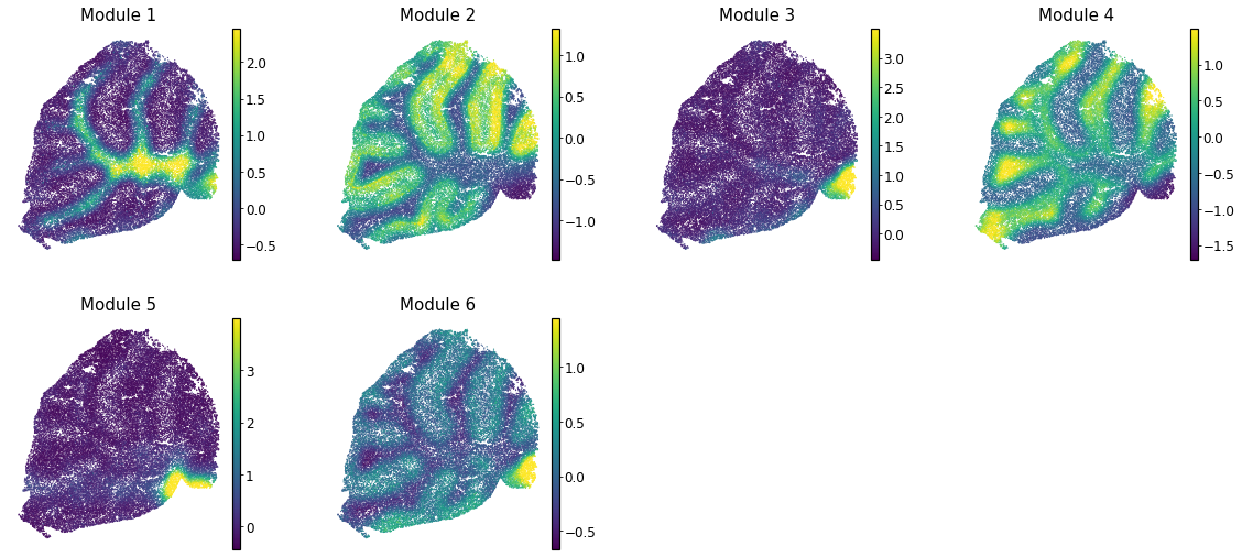
Compute summary per-cell module scores
Finally, summary per-cell scores can be computed for a module. This is useful for visualizng the general pattern of expression for genes in a module.
module_scores = hs.calculate_module_scores()The output is a pandas DataFrame (cells x modules) and is also saved in hs.module_scores
module_scores:
| 1 | 2 | 3 | 4 | 5 | |
|---|---|---|---|---|---|
| AAACCCAAGGCCTAGA-1 | 0.785 | -2.475 | -1.407 | -0.681 | -1.882 |
| AAACCCAGTCGTGCCA-1 | -5.76 | 5.241 | 6.931 | 1.928 | 4.317 |
| AAACCCATCGTGCATA-1 | -2.619 | 3.572 | 0.143 | 1.832 | 1.585 |
| AAACGAAGTAATGATG-1 | -8.778 | 4.012 | 6.927 | 1.181 | 3.882 |
| AAACGCTCATGCACTA-1 | 2.297 | -2.517 | -1.421 | -1.102 | -1.547 |
| ... | ... | ... | ... | ... | ... |
These can then be plotted onto other visual representations of the cells. For example, for spatial modules (from data in Rodriques et al, 2019) this looks like: