Command Obfuscation Detection using Deep Learning
Command obfuscation is a technique to make a piece of code intentionally hard-to-read, but still execute the same functionality. Malicious attackers often abuse obfuscation to make their malicious software (malware) evasive to traditional malware detection techniques. This creates a headache for defenders since attackers can create a virtually infinite number of ways to obfuscate their malware. Traditional malware detection techniques are often rule-based, rendering them inflexible to new types of malware and obfuscation techniques. Deep learning has been used in various domains to create models that are dynamic and can adapt to new types of information. Our project uses deep learning techniques to detect command obfuscation.
- Blog post: https://medium.com/adobetech/using-deep-learning-to-better-detect-command-obfuscation-965b448973e0
- Pip package: https://pypi.org/project/obfuscation-detection/
Usage - Quick Installation
You can install our package through pip!
pip install obfuscation-detectionThis is a basic usage of our package:
import obfuscation_detection as od

oc = od.ObfuscationClassifier(od.PlatformType.ALL)
commands = ['cmd.exe /c "echo Invoke-DOSfuscation"',
            'cm%windir:~ -4, -3%.e^Xe,;^,/^C",;,S^Et ^^o^=fus^cat^ion&,;,^se^T ^ ^ ^B^=o^ke-D^OS&&,;,s^Et^^ d^=ec^ho I^nv&&,;,C^Al^l,;,^%^D%^%B%^%o^%"',
            'cat /etc/passwd']
classifications = oc(commands)

# 1 is obfuscated, 0 is non-obfuscated
print(classifications) # [0, 1, 0]
Model Architecture
Input
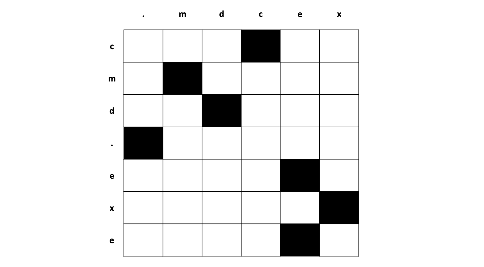
The input into the model is a single command from the command line. We represent a single command by each character individually. Each character is represented by a one-hot vector, a vector where all the values are 0 except for one index and the one index represented which character it is. We also include an extra case bit to differentiate between uppercase and lowercase characters. We found the frequency of the most common characters in our dataset and found 73 characters. With the case bit, each character one-hot vector is 74-dimensional. Each command is also represented by its first 4096 characters. If the command is longer than 4096 characters, the rest is cut off and if the command is shorter, then the rest is padded with zero's. Therefore, the input to our model is a 74x4096 matrix.
Below is a simplified illustration of the input matrix, where the vertical axis represents the command and the horizontal axis represents the one-hot encoding.

Model - it's a CNN
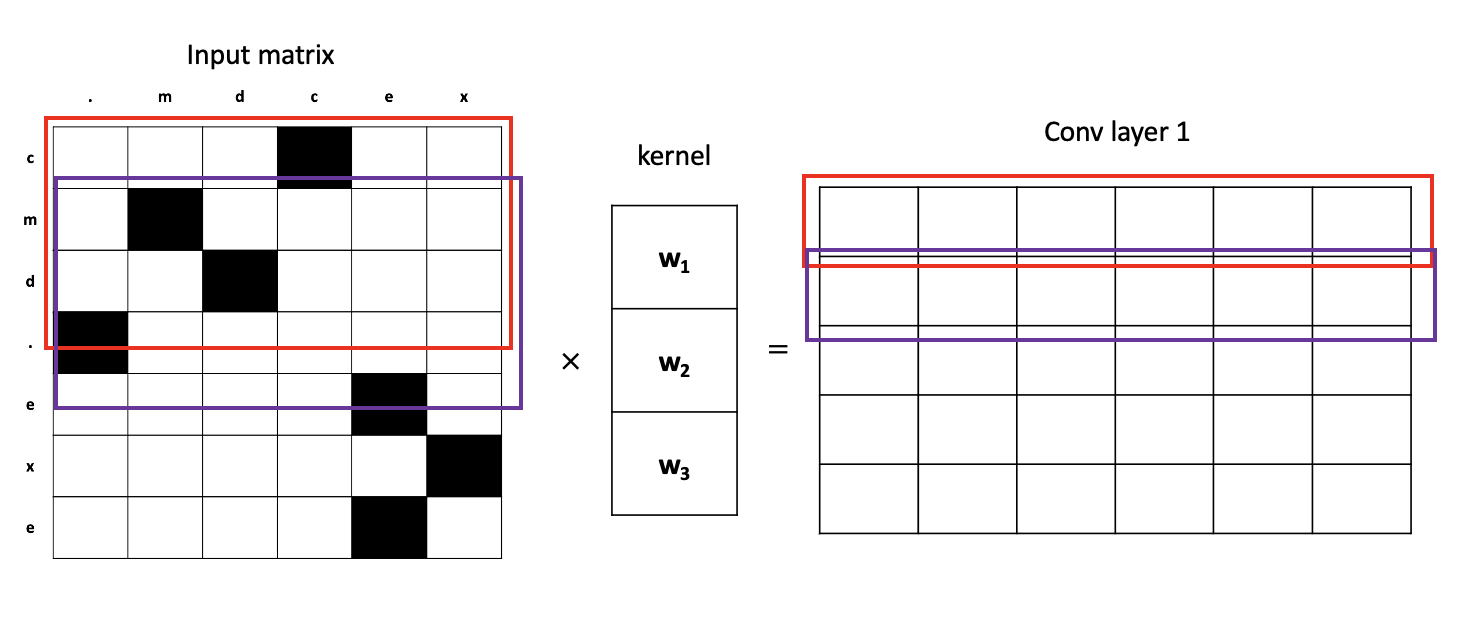
Our model is a character-level deep convolutional neural network (CNN). What does this mean? Let's look at the first layer, turning our input matrix into a convolutional layer (conv layer). We look at a few characters that are close to each other, multiply some weights onto these characters, and come out with a resulting vector. In the image below, we first look at 3 characters depicted by the left red box. We multiply these 3 characters by the kernel weight vector and it results in the right red box vector. We continue this process for all 3-character blocks next to each other, depicted by the purple box. We stack all these resulting vectors to form a matrix that results in our 1st conv layer.

The 1st conv layer now contains a matrix of vectors, where each row carries semantic meaning of 3 characters. We continue this process of applying convolutions, thereby increasing the "window size" each row in the matrix sees. If we apply one more layer of convolutions to our example, the next conv layer (conv layer 2) will contain rows where each row carries semantic meaning of 5 characters. The higher the layer, the bigger the window size is. The bigger the window size, the more semantic meaning each row the conv layer can carry.

We apply this process of convolutions with weights to extract features from the input. After we apply a couple layers of convolutions, we finally make a decision by taking an average of the CNN's output (final layer). This average is then run through a final fully connected (FC) layer to make the final output which is a 2-dimensional vector. The first dimension is the model's prediction on how non-obfuscated the command is. The second dimension is the model's prediction on how obfuscated the command is. We take the max of these two dimensions to decide whether or not the command is obfuscated. For example, a prediction that the command is not obfuscated is <1, 0> while a prediction that the command is obfuscated is <0, 1>.

Model - and it's also a ResNet
Our model also has aspects of a ResNet. Since we are using this CNN for a language task, we found it natural to apply the same types of methods in RNNs as CNNs. Now you might ask why not just use RNNs? Well, in a nutshell, CNNs are faster than RNNs. CNNs are able to do parallel computations while RNNs rely on the previous sequence before it calculates the current sequence. Since our task is character-level, we don't require this task to be a sequence task. Therefore, we believe CNNs better capture the semantics of this task.
So, what ResNet components are there? Here they are:
- Residual connection: The output of each layer are summed up for each layer, then this residual block is added to the final CNN output layer. This helps solve the problem of vanishing gradients in models with many layers.
- Skip connection: The output of the previous layer is added onto the output of the current layer. This is so if any layer hurts the model architecture, it can be skipped by regularization.
- Gated activation function: For each CNN layer, we apply a sigmoid activation on half the filters and a tanh activation on the other half, then element-wise multiply these two activations together. This has shown better performance in signal-based applications, such as WaveNet.

Upgrading our model from a plain CNN to a CNN + ResNet gave us much better performance!
Results
Overall, our model performs very well on windows and linux commands!
Development
Pre-requisites
-
Install python dependencies:
pip install -r requirements.txt -
Make empty directories for runtime
mkdir data mkdir data/prep mkdir data/processed_tensors mkdir data/processed_csv mkdir data/scripts mkdir models -
Download the Powershell Corpus: https://aka.ms/PowerShellCorpus. Unzip the file into the
datadirectory -
Download PS corpus labels: https://github.com/danielbohannon/Revoke-Obfuscation. Clone the repo in the same-level directory as this repo. The labels are found in the
DataSciencefolder. -
Download DOSfuscated commands: https://github.com/danielbohannon/Invoke-DOSfuscation/tree/master/Samples. Download the four
STATIC_#_of_4_*files and put them inside thedatadirectory. -
We also use internal Adobe command line executions as a bulk of our training data. We may not release this dataset to the public, so we encourage you to either not exclude this dataset or find an open-source command prompt dataset on the internet.
Data Prep
cd data-prep, then run the following python scripts in order:
-
python char_frequency.py: creates a .txt file of each charcter's frequency in the dataset -
python char_dict.py: creates a python dict of the most common characters mapped to a numeric index -
python ps_data_preprocess.py: creates dataset for the powershell corpus dataset -
python dos_data_preprocess.py: creates dataset for the DOSfuscated commands -
python hubble_data_preprocess.pyandpython cb_data_preprocess.py: creates dataset for internal Adobe data. Replace this step with other data you may find on the internet. -
python win_data_preprocess.py: creates train/dev/test tensor split by accumulating all windows data. -
python linux_obf_data_preprocess.py: load internal Adobe linux commands and obfuscate them -
python linux_data_preprocess.py: creates train/dev/test tensor split with all linux data -
python all_data_preprocess.py: combines windows and linux train/dev/test sets together for a big train/dev/test dataset.
Usage
cd ../scripts, then run python train.py with the given options!
train.py:
--model- choose a model architecture--model-file- filename of model checkpoint--cuda-device- which cuda device to use- Choose one of:
--reset- start training from scratch--eval- evaluate on best checkpoint on train/dev--analyze- create fp/fn files from dev--run- run on real scripts ontest-scriptsdir--test- run model on test set- none - continue training model from checkpoint
models.py: contains the different model architectures we experimented with
Examples
Training model:
- From scratch:
python train.py --model resnet --model_file resnet.pth --reset - From checkpoint:
python train.py --model resnet --model_file resnet.pth
Eval model: python train.py --model resnet --model_file resnet.pth --eval
Test model: python train.py --model resnet --model_file resnet.pth --test
Running model on new data:
- Put each separate script/command in its own file
- Put all script/command files in a new dir
test-scripts - Run
python train.py --model resnet --model_file resnet.pth --run
We have included our best model in models/best-resnet-*.pth!
Contributing
Contributions are welcomed! Read the Contributing Guide for more information.
Licensing
This project is licensed under the Apache V2 License. See LICENSE for more information.