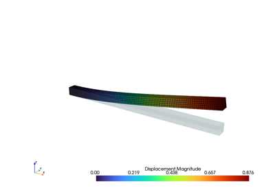
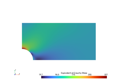
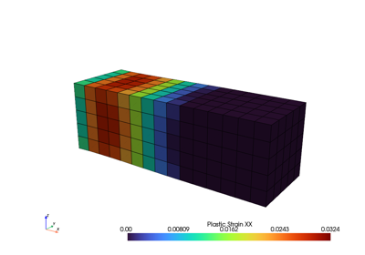
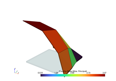
Finite element analysis for continuum mechanics of solid bodies.

PyPI - Downloads

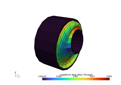
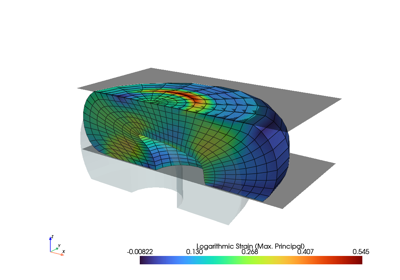
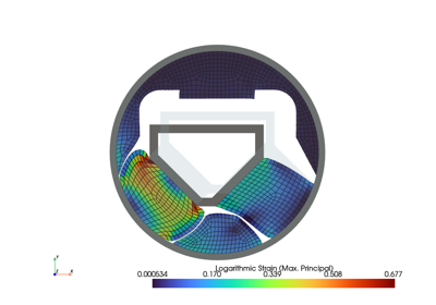
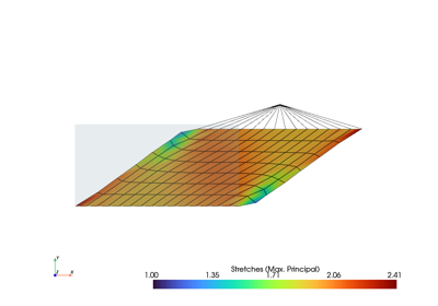
FElupe is a Python 3.9+ 🐍 finite element analysis package 📦 focusing on the formulation and numerical solution of nonlinear problems in continuum mechanics of solid bodies 🔧. This package is intended for scientific research 💻, but is also suitable for running nonlinear simulations 🚂 in general 🏎️. In addition to the transformation of general weak forms into sparse vectors and matrices, FElupe provides an efficient high-level abstraction layer for the simulation of the deformation of solid bodies.

Highlights

[x] 100% Python package built with NumPy and SciPy
[x] easy to learn and productive high-level API
[x] nonlinear deformation of solid bodies
[x] interactive views on meshes, fields and solid bodies (using PyVista)
[x] typical finite elements
[x] cartesian, axisymmetric, plane strain and mixed fields
[x] hyperelastic material models with automatic differentiation

Efficient NumPy-based math is realized by element-wise operating trailing axes [1]. The finite element method, as used in FElupe, is based on [2], [[3]]() and [4]. Related scientific articles are listed in the sections of the API reference.

[!NOTE] FElupe is a combination of FE (finite element) and the german word Lupe 🔍 (magnifying glass) as a synonym for getting an insight 📖 how a finite element analysis code 🧮 looks like under the hood 🕳️.

Installation

Install Python, fire up 🔥 a terminal and run 🏃

pip install felupe[all]

The documentation covers more details, like required and optional dependencies and how to install the latest development version.

Getting Started

This tutorial covers the essential high-level parts of creating and solving problems with FElupe. As an introductory example 👨‍🏫, a quarter model of a solid cube with hyperelastic material behaviour is subjected to a uniaxial elongation applied at a clamped end-face.

First, let’s import FElupe and create a meshed cube out of hexahedron cells with a given number of points per axis. A numeric region, pre-defined for hexahedrons, is created on the mesh. A vector-valued displacement field is initiated on the region. Next, a field container is created on top of this field.

A uniaxial load case is applied on the displacement field stored inside the field container. This involves setting up symmetry planes as well as the absolute value of the prescribed displacement at the mesh-points on the right-end face of the cube. The right-end face is clamped 🛠️: only displacements in direction x are allowed. The dict of boundary conditions for this pre-defined load case are returned as boundaries and the partitioned degrees of freedom as well as the external displacements are stored within the returned dict loadcase.

An isotropic pseudo-elastic Ogden-Roxburgh Mullins-softening model formulation in combination with an isotropic hyperelastic Neo-Hookean material formulation is applied on the displacement field of a nearly-incompressible solid body.

A step generates the consecutive substep-movements of a given boundary condition. The step is further added to a list of steps of a job 👩‍💻 (here, a characteristic-curve 📈 job is used). During evaluation ⏳, each substep of each step is solved by an iterative Newton-Rhapson procedure ⚖️. The solution is exported after each completed substep as a time-series ⌚ XDMF file. Finally, the result of the last completed substep is plotted.

For more details beside this high-level code snippet, please have a look at the 📝 documentation.

import felupe as fem

mesh = fem.Cube(n=6)
region = fem.RegionHexahedron(mesh)
field = fem.FieldContainer([fem.Field(region, dim=3)])

boundaries, loadcase = fem.dof.uniaxial(field, clamped=True)

umat = fem.OgdenRoxburgh(material=fem.NeoHooke(mu=1), r=3, m=1, beta=0.1)
solid = fem.SolidBodyNearlyIncompressible(umat, field, bulk=5000)

move = fem.math.linsteps([0, 1, 0, 1, 2, 1], num=5)
step = fem.Step(items=[solid], ramp={boundaries["move"]: move}, boundaries=boundaries)

job = fem.CharacteristicCurve(steps=[step], boundary=boundaries["move"])
job.evaluate(filename="result.xdmf")
fig, ax = job.plot(
    xlabel="Displacement $u$ in mm $\longrightarrow$",
    ylabel="Normal Force $F$ in N $\longrightarrow$",
)

solid.plot("Principal Values of Cauchy Stress").show()

Curve Solid Body

Documentation

The documentation is located here.

Extension Packages

The capabilities of FElupe may be enhanced with extension packages created by the community.

Package	Description
hyperelastic	Constitutive hyperelastic material formulations
matadi	Material Definition with Automatic Differentiation (AD)
tensortrax	Differentiable Tensors based on NumPy Arrays
feplot	A visualization tool for FElupe

Testing

To run the FElupe unit tests, check out this repository and type

tox

Scientific Publications

A list of articles in which is involved. If you use FElupe in your scientific work, please star this repository, cite it and add your publication to this list.

A. Dutzler, C. Buzzi, and M. Leitner, "Nondimensional translational characteristics of elastomer components", Journal of Applied Engineering Design and Simulation, vol. 1, no. 1. UiTM Press, Universiti Teknologi MARA, Sep. 21, 2021. doi: 10.24191/jaeds.v1i1.20.
C. Buzzi, A. Dutzler, T. Faethe, J. Lassacher, M. Leitner, and F.-J. Weber, "Development of a tool for estimating the characteristic curves of rubber-metal parts", in Proceedings of the 12th International Conference on Railway Bogies and Running Gears, 2022 (ISBN 978-963-9058-46-0).
J. Torggler, A. Dutzler, B. Oberdorfer, T. Faethe, H. Müller, C. Buzzi, and M. Leitner, "Investigating Damage Mechanisms in Cord-Rubber Composite Air Spring Bellows of Rail Vehicles and Representative Specimen Design", Applied Composite Materials. Springer Science and Business Media LLC, Aug. 22, 2023. doi: 10.1007/s10443-023-10157-1. Simulation-related Python scripts are available on GitHub at adtzlr/fiberreinforcedrubber.

Changelog

All notable changes to this project will be documented in this file. The format is based on Keep a Changelog, and this project adheres to Semantic Versioning.

References

[1] T. Gustafsson and G. McBain, "scikit-fem: A Python package for finite element assembly", Journal of Open Source Software, vol. 5, no. 52. The Open Journal, p. 2369, Aug. 21, 2020. .

[2] J. Bonet and R. D. Wood, "Nonlinear Continuum Mechanics for Finite Element Analysis". Cambridge University Press, Mar. 13, 2008. .

[[3]]() K. J. Bathe, "Finite Element Procedures". 2006, isbn: 978-0-9790049-0-2.

[4] O. C. Zienkiewicz, R. L. Taylor and J. Z. Zhu, "The Finite Element Method: its Basis and Fundamentals". Elsevier, 2013. .

License

This program is free software: you can redistribute it and/or modify it under the terms of the GNU General Public License as published by the Free Software Foundation, either version 3 of the License, or (at your option) any later version.

This program is distributed in the hope that it will be useful, but WITHOUT ANY WARRANTY; without even the implied warranty of MERCHANTABILITY or FITNESS FOR A PARTICULAR PURPOSE. See the GNU General Public License for more details.

You should have received a copy of the GNU General Public License along with this program. If not, see https://www.gnu.org/licenses/.

adtzlr / felupe

readme