PyDEns

PyDEns is a framework for solving Ordinary and Partial Differential Equations (ODEs & PDEs) using neural networks. With PyDEns one can solve

PDEs & ODEs from a large family including heat-equation, poisson equation and wave-equation
parametric families of PDEs
PDEs with trainable coefficients.

This page outlines main capabilities of PyDEns. To get an in-depth understanding we suggest you to also read the tutorial.

Getting started with PyDEns: solving common PDEs

Let's solve poisson equation

using simple feed-forward neural network. Let's start by importing Solver-class along with other needed libraries:

from pydens import Solver, NumpySampler
import numpy as np
import torch

You can now set up a PyDEns-model for solving the task at hand. For this you need to supply the equation into a Solver-instance. Note the use of differentiation token D:

# Define the equation as a callable.
def pde(f, x, y):
    return D(D(f, x), x) + D(D(f, y), y) - 5 * torch.sin(np.pi * (x + y))

# Supply the equation, initial condition, the number of variables (`ndims`)
# and the configration of neural network in Solver-instance.
solver = Solver(equation=pde, ndims=2, boundary_condition=1,
                layout='fa fa fa f', activation='Tanh', units=[10, 12, 15, 1])

Note that we defined the architecture of the neural network by supplying layout, activation and units parameters. Here layout configures the sequence of layers: fa fa fa f stands for fully connected architecture with four layers and three activations. In its turn, units and activation cotrol the number of units in dense layers and activation-function. When defining neural network this way use ConvBlock from BatchFlow.

It's time to run the optimization procedure

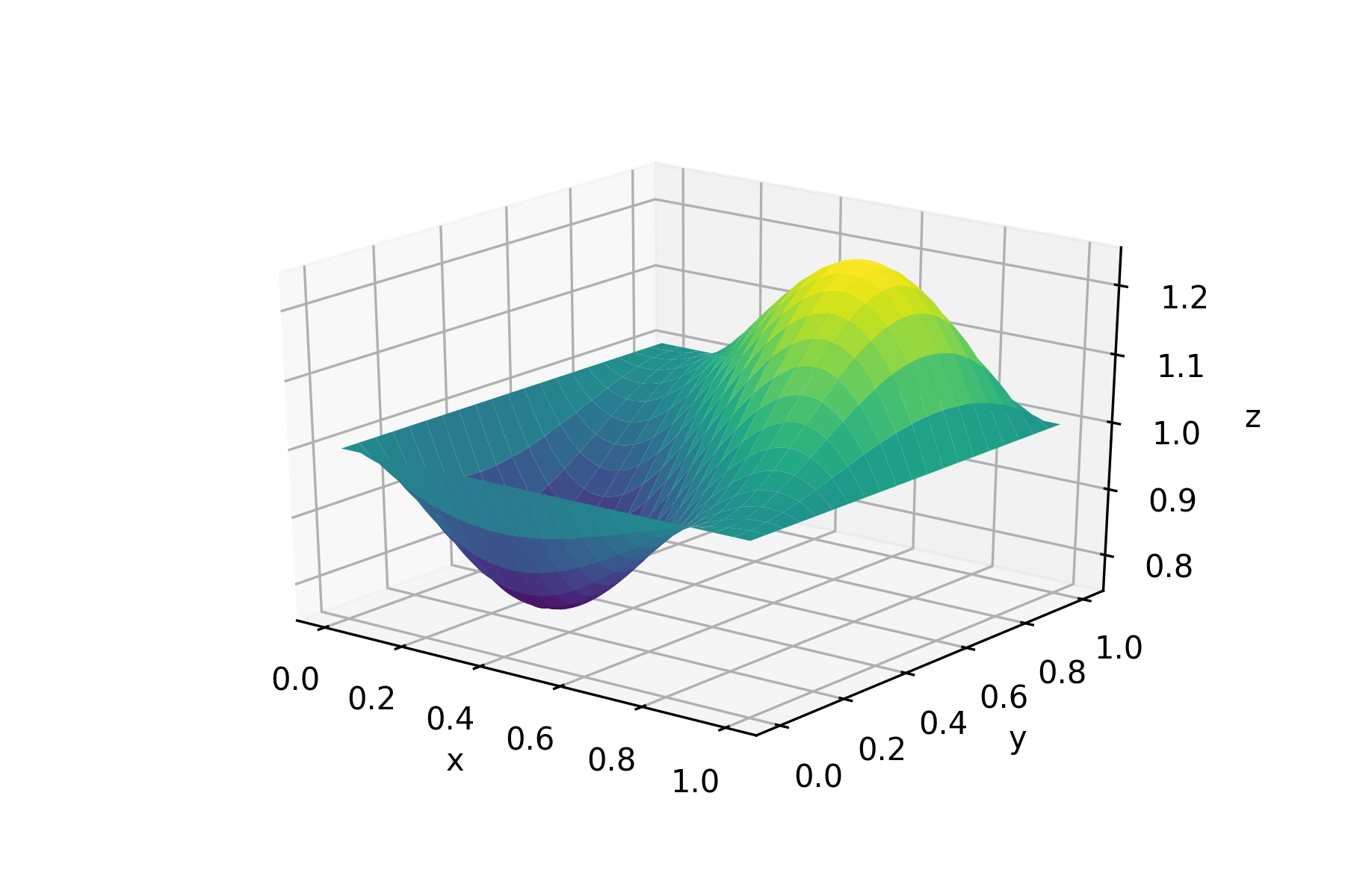
solver.fit(batch_size=100, niters=1500)

in a fraction of second we've got a mesh-free approximation of the solution on [0, 1]X[0, 1]-square:

Going deeper into PyDEns-capabilities

PyDEns allows to do much more than just solve common PDEs: it also deals with (i) parametric families of PDEs and (ii) PDEs with trainable coefficients.

Solving parametric families of PDEs

Consider a family of ordinary differential equations

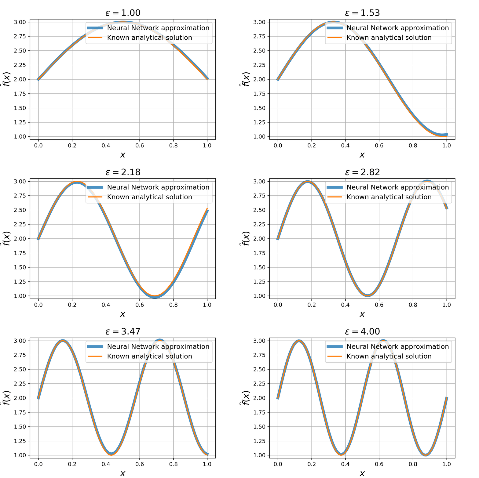
Clearly, the solution is a sin wave with a phase parametrized by ϵ:

Solving this problem is just as easy as solving common PDEs. You only need to introduce parameter e in the equation and supply the number of parameters (nparams) into a Solver-instance:

def odeparam(f, x, e):
    return D(f, x) - e * np.pi * torch.cos(e * np.pi * x)

# One for argument, one for parameter
s = NumpySampler('uniform') & NumpySampler('uniform', low=1, high=5)

solver = Solver(equation=odeparam, ndims=1, nparams=1, initial_condition=1)
solver.fit(batch_size=1000, sampler=s, niters=5000, lr=0.01)
# solving the whole family takes no more than a couple of seconds!

Check out the result:

Solving PDEs with trainable coefficients

With PyDEns things can get even more interesting! Assume that the initial state of the system is unknown and yet to be determined:

Of course, without additional information, the problem is undefined. To make things better, let's fix the state of the system at some other point:

Setting this problem requires a slightly more complex configuring. Note the use of V-token, that stands for trainable variable, in the initial condition of the problem. Also pay attention to the additional constraint supplied into the Solver instance. This constraint binds the final solution to zero at t=0.5:

def odevar(u, t):
    return D(u, t) - 2 * np.pi * torch.cos(2 * np.pi * t)
def initial(*args):
    return V('init', data=torch.Tensor([3.0]))

solver = Solver(odevar, ndims=1, initial_condition=initial,
                constraints=lambda u, t: u(torch.tensor([0.5])))

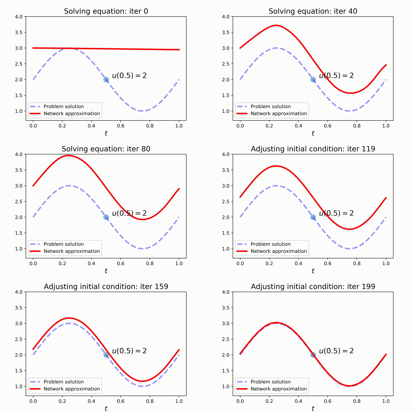
When tackling this problem, pydens will not only solve the equation, but also adjust the variable (initial condition) to satisfy the additional constraint. Hence, model-fitting comes in two parts now: (i) solving the equation and (ii) adjusting initial condition to satisfy the additional constraint. Inbetween the steps we need to freeze layers of the network to adjust only the adjustable variable:

solver.fit(batch_size=150, niters=100, lr=0.05)
solver.model.freeze_layers(['fc1', 'fc2', 'fc3'], ['log_scale'])
solver.fit(batch_size=150, niters=100, lr=0.05)

Check out the results:

Installation

First of all, you have to manually install pytorch, as you might need a certain version or a specific build for CPU / GPU.

Stable python package

With modern pipenv

pipenv install pydens

With old-fashioned pip

pip3 install pydens

Development version

pipenv install git+https://github.com/analysiscenter/pydens.git

pip3 install git+https://github.com/analysiscenter/pydens.git

Installation as a project repository:

Do not forget to use the flag --recursive to make sure that BatchFlow submodule is also cloned.

git clone --recursive https://github.com/analysiscenter/pydens.git

In this case you need to manually install the dependencies.

Citing PyDEns

Please cite PyDEns if it helps your research.

Roman Khudorozhkov, Sergey Tsimfer, Alexander Koryagin. PyDEns framework for solving differential equations with deep learning. 2019.

@misc{pydens_2019,
  author       = {Khudorozhkov R. and Tsimfer S. and Koryagin. A.},
  title        = {PyDEns framework for solving differential equations with deep learning},
  year         = 2019
}

analysiscenter / pydens

readme