Table of Contents
Introduction
Automated Local Phylogenomic Analyses, or ALPHA, is a python-based application that provides an intuitive user interface for phylogenetic analyses and data visualization. It has four distinct modes that are useful for different types of phylogenetic analysis: RAxML, File Converter, MS Comparison, and D-statistic.

RAxML mode gives users a front-end to interact with RAxML (STAMATAKIS 2014a) for Maximum Likelihood based inference of large phylogenetic trees. ALPHA’s RAxML mode allows one to use RAxML to automatically perform sliding window analysis over an inputted alignment. Users are able to select from a plethora of options in performing their analysis, including: window size, window offset, and number of bootstraps. In this mode, users are able to produce a variety of graphs to help understand their genomic alignment and interpret the trees outputted by RAxML. These graph options include: a tree visualization of the top topologies, scatter plot of windows to their topologies, frequency of top topologies, a line graph of windows to the percent of informative sites, and a heat map of the informative sites. RAxML mode also provides support for calculating two statistics based on the trees produced within each window as compared to an overall species tree: Robinson-Foulds distance and the probability of a gene tree given a species tree.
The file converter in ALPHA provides a user interface for a Biopython AlignIO file converter function. It allows users to convert between twelve popular genome alignment file types. RAxML mode only accepts phylip-sequential format. MS Comparison mode allows users to perform an accuracy comparison between a “truth file” and one or more files in MS format or the results of RAxML mode. With D-statistic mode, users can compute Patterson’s D-statistic for determining introgression in a four taxa alignment. D-statistic mode produces a scatter plot of the value of the D-statistic across sliding windows as well as the value of the D-statistic across the entire alignment.
Requirements
ALPHA currently runs on both Mac and Windows operating systems and selects the proper operating system automatically. Python 2.7.13 and Java are required for this GUI, along with the additional libraries: BioPython, DendroPy, ETE, Matplotlib, natsort, PIL, PyQt4, ReportLab, SciPy, Statistics, and SVGUtils. RAxML is also required for performing analysis in RAxML mode.
Avoid special characters, such as diacritics, spaces, and punctuation other than dots (“.”) and underscores (“_”) in the names of the ALPHA folder and all input files.
Analysis Modes
RAxML
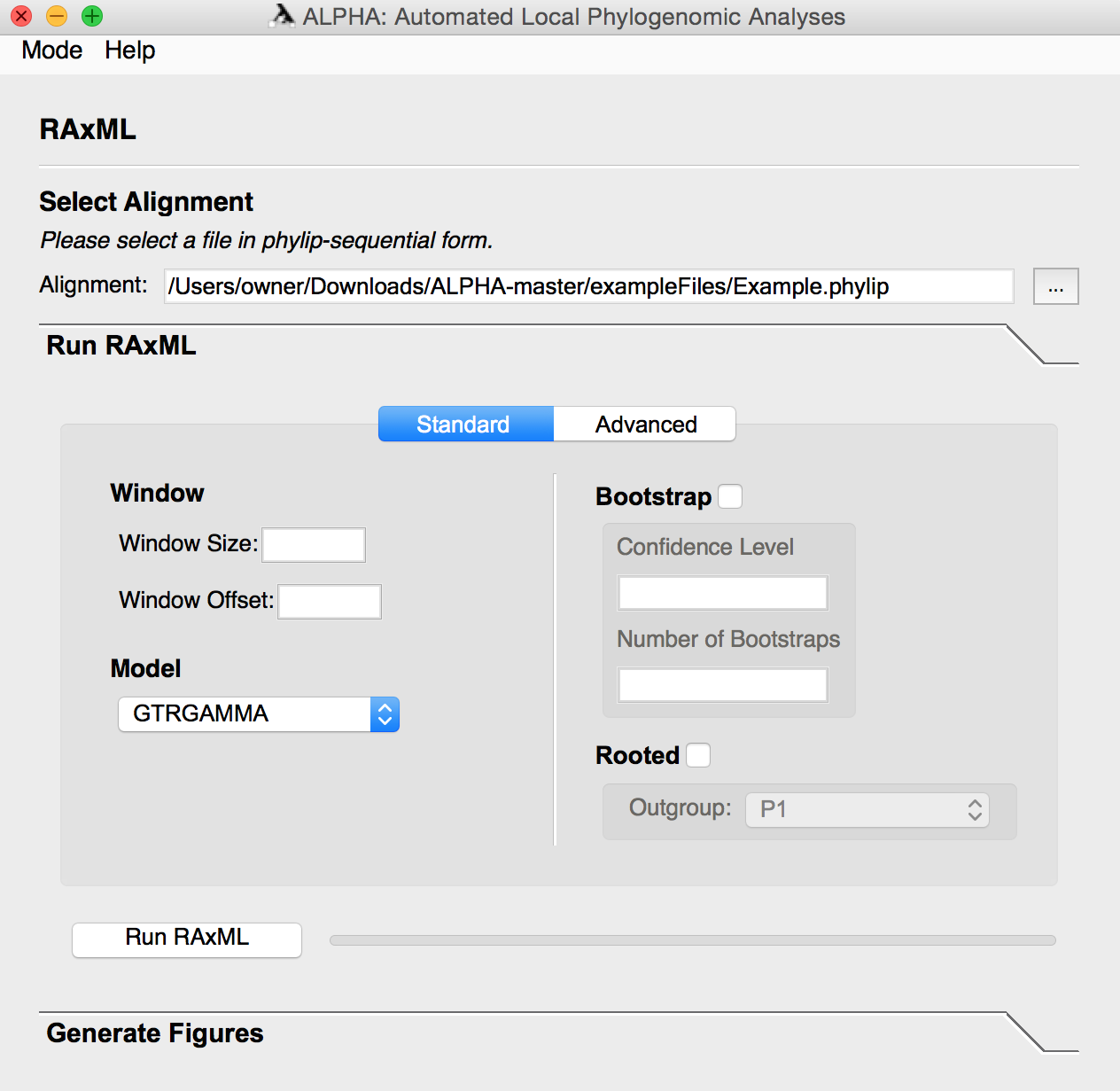
In RAxML mode, there are two analysis sections containing preferences for adjusting the statistics. In the Run RAxML section, the user selects a file in phylip-sequential format and modifies the options within the Standard or Advanced RAxML settings to fit their preferences.
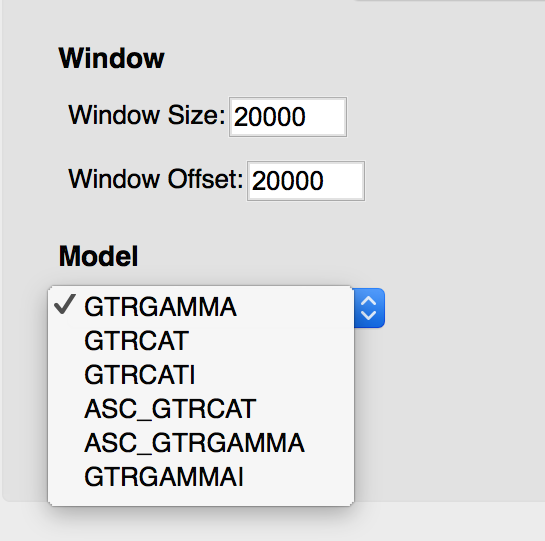
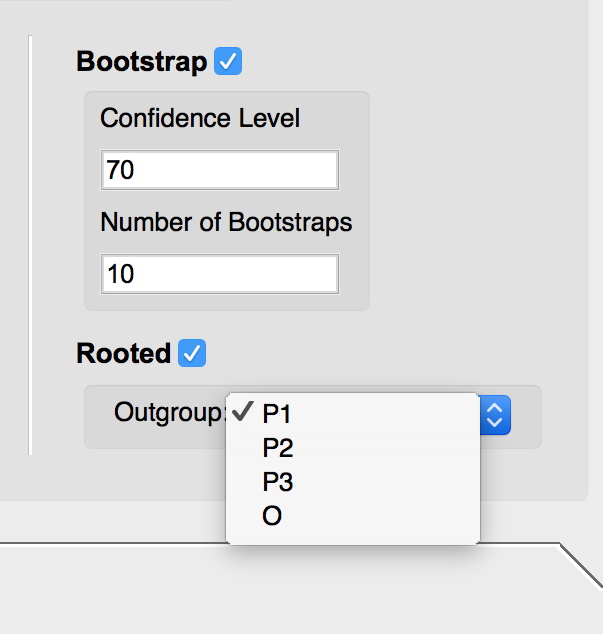
In standard mode, the window size, window offset, and the number of top topologies to be analyzed can be inputted manually as integers greater than one. The model type can be selected from six popular types. Bootstrapping can also be selected; if it is, the user can input the confidence level and the number of bootstraps to be performed. The user can also choose to root the tree at a specific outgroup in the input file.
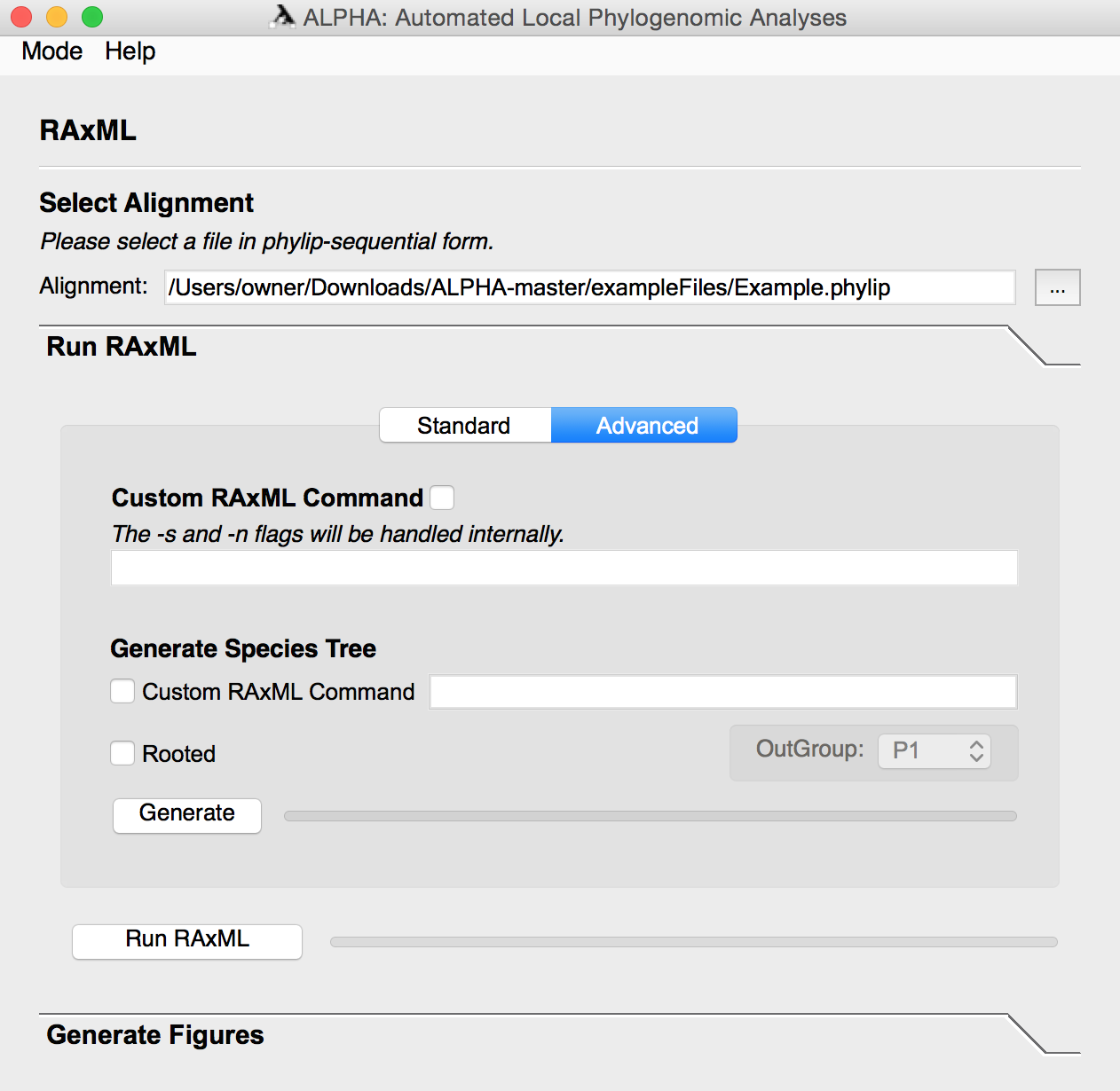
In advanced mode, the user can input a custom RAxML command in which the -s and -n flags are handled internally. A rooted or unrooted species tree can also be generated in this mode using a custom RAxML command or by simply clicking Generate, which runs RAxML on the entire alignment.
For more information regarding RAxML and its commands see the RAxML manual.
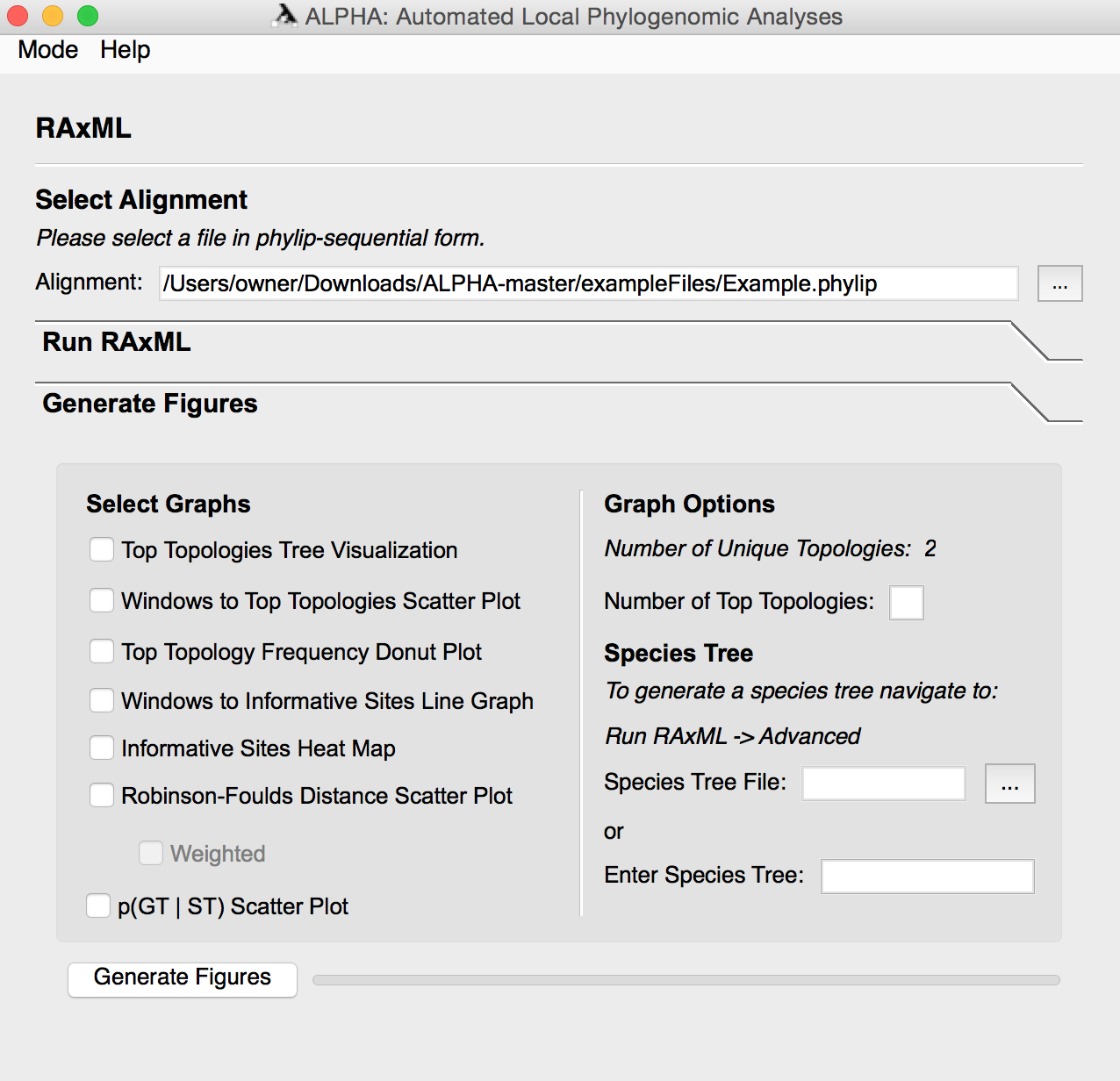
After running RAxML, the user can enter the Generate Figures section and select any of the following: Top Topologies Tree Visualization, Windows to Top Topologies Scatter Plot, Top Topology Frequency Donut Plot, Windows to Informative Sites Line Graph, Informative Sites Heat Map, the weighted and/or unweighted Robinson-Foulds Distance Scatter Plot, and the Probability of a Gene Tree given the Species Tree Scatter Plot. The user can also specify how many top toplogies they want to analyze and input a species tree file or string in Graph Options.
The Top Topologies Tree Visualization generates an image containing the most frequently occuring local phylogenies generated by running RAxML on windows of the previously specified size. The visualization also includes the number of times each topology occurs.
The Windows to Top Topologies Scatter Plot shows the windows at which each local phylogeny occurs and depicts the x-axis as the window number and the y-axis as the topology.
The Top Topology Frequency Donut Plot is a graph showing the number of times each topology occurs; topologies differing from the top topologies are lumped together and categorized as “Other.”
Generate the Top Topologies Tree Visualization, Windows to Top Topologies Scatter Plot, and Top Topology Frequency Donut Plot at the same time to ensure that the colors of the topologies correspond with the colors used within the plots.
The Windows to Informative Sites Line Graph shows how the percent of informative sites differs across each window. Windows are on the x-axis, and the Percent of Informative Sites is on the y-axis.
The Informative Sites Heat Map depicts the informativeness of each site in the data. If a site is informative, there is a black line. The more informative the site, the thicker the line in the heat map.
The Robinson-Foulds Distance Scatter Plot depicts the Robinson-Foulds distance between the local phylogeny and the species tree. The user can choose to generate the Weighted Robinson-Foulds Distance Scatter Plot, which takes branch lengths into account, or they can generate both the weighted and unweighted plots by not checking the Weighted option.
The Probability of A Gene Tree Given the Species Tree Scatter Plot shows the probability of the local phylogeny at a window actually occurring given the inputted species tree.
File Converter
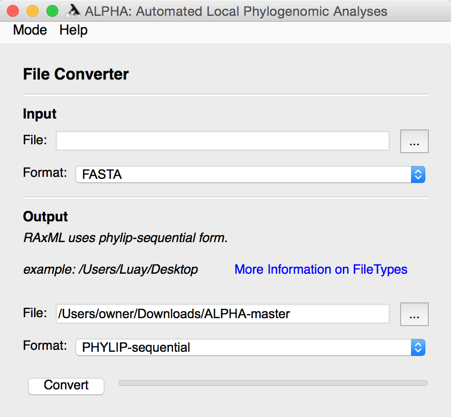
File Converter mode allows the user to select a file containing DNA alignments in one of twelve popular formats and convert them to a different file format. After selecting the input file and its format, the user must specify the output file’s name and location along with the desired format.
For more information regarding file types see BioPython AlignIO.
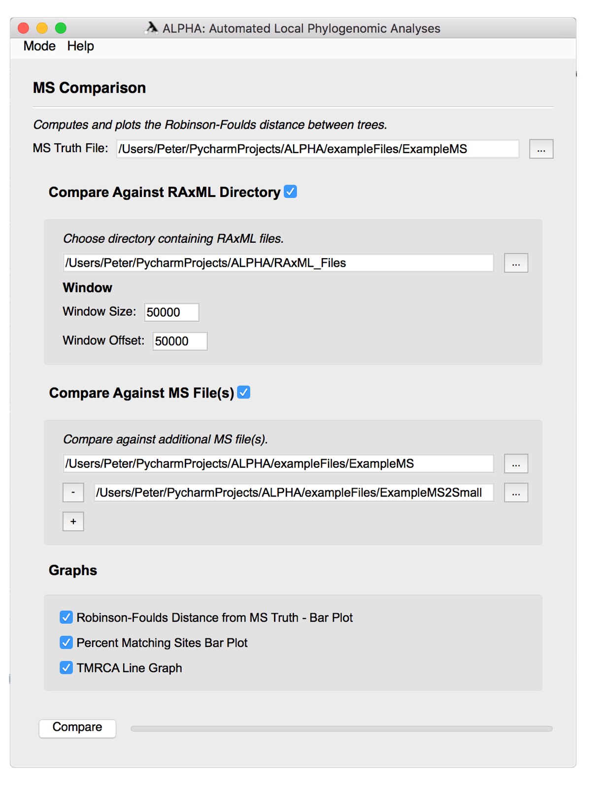
MS Comparison
In MS Comparison mode, the user can specify an MS truth file and the RAxML directory and/or other MS files to compare it to . This mode has options to generate figures for Robinson-Foulds Distance From MS Truth Bar Plot, Percent Matching Sites Bar Plot, and TMRCA Line Graph.
When comparing against the RAxML directory, the user has the option to input the directory containing the RAxML files and choose the window size and offset. This function is meant to be used after performing sliding window analysis in ALPHA’s RAxML mode.
When comparing the truth file to other MS files, the user can input multiple MS files for comparison.
The Robinson-Foulds Distance from MS Truth Bar Plot depicts the total difference between the trees in the truth file and other files chosen for comparison.
The Percent Matching Sites Bar Plot shows the percentage of sites in the comparison file(s) that contain trees that match the truth file for both weighted and unweighted analyses. The Robinson-Foulds distance is used to determine if a tree is considered a match or not.
The TMRCA Line Graph shows the tree height over each site when comparing the truth files and other files. This figure is meant to depict to the differences in the time to most recent common ancestor (TMRCA) between each file.

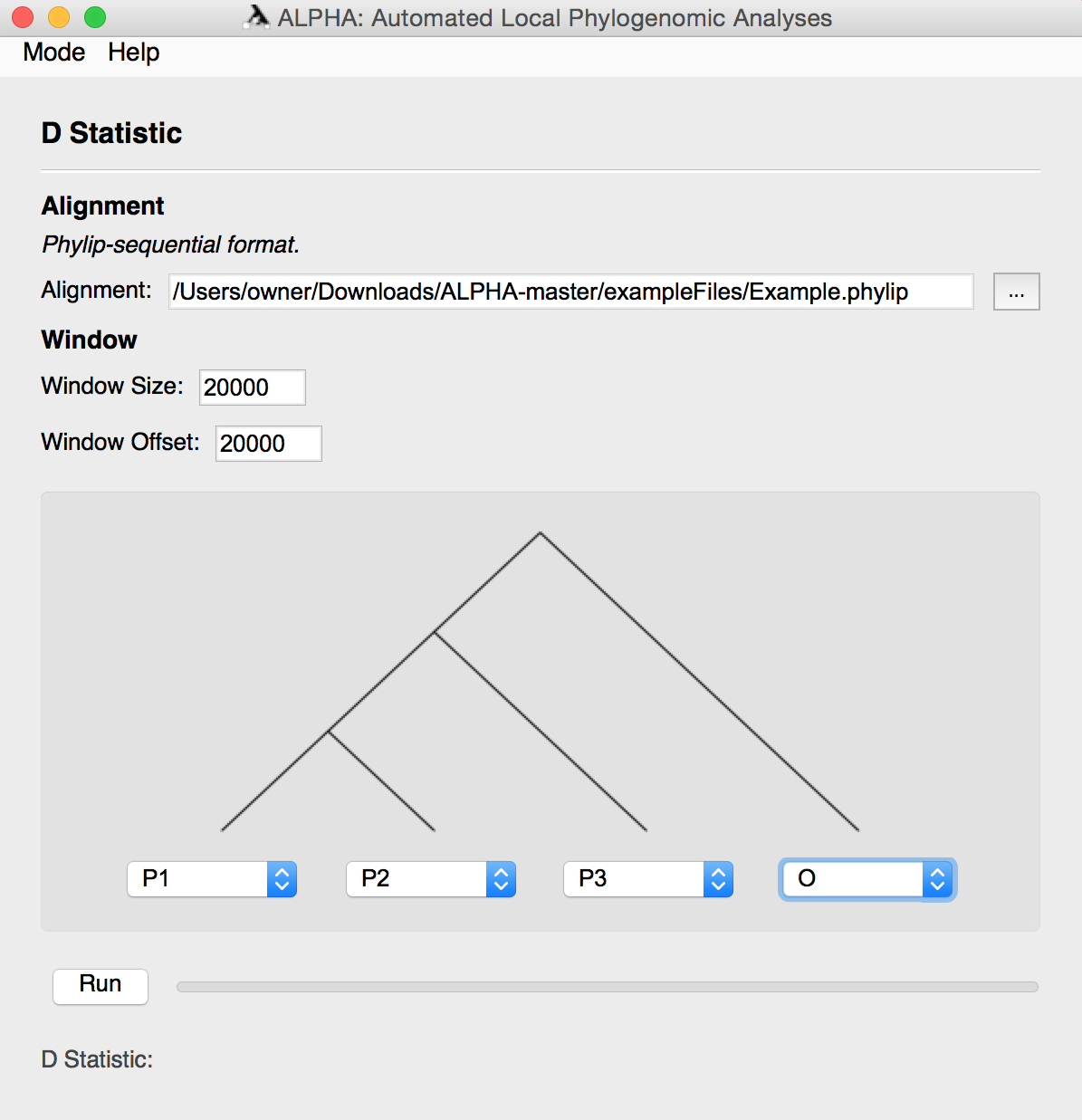
D-statistic
D-statistic mode allows the user to input an alignment file in phylip-sequential format, choose the window size and offset, and select the location of each outgroup in the tree visual. This mode then generates the overall D-statistic and a scatter plot in which the x-axis is the window number, and the y-axis is the D-statistic value computed for that window.

For further reading on the D Statistic and its usage see: \ Green et al. (2010), Durand et al. (2011), Martin et al. (2014)
D-gen-statistic
UPDATE 3/14/19:
THE D GEN ALGORITHM AND GUI HAVE UNDERGONE A MAJOR OVERHAUL. THESE INSTRUCTIONS WILL BE UPDATED VERY SOON ALONGSIDE AN ACCOMPANYING PAPER DETAILING THE NEW ALGORITHM. THANK YOU FOR YOUR PATIENCE.
ALPHA’s generalized D statistic has many different inputs to cover a range of user preferences. This section will go over each input and its usage in both the user interface and command line script.
To run the command line version of the generalized D statistic cd into the CommandLineFiles directory and use the following command with one’s desired parameters. All possible parameters are listed below along with their default values for the command line script. Note: not all of these parameters can not be called at the same time.
python -c "from CalculateGeneralizedDStatistic import *; calculate_generalized(alignments, species_tree=None, reticulations=None, outgroup=None, window_size=100000000000, window_offset=100000000000, verbose=False, alpha=0.01, useinv=False, useDir=False, directory="", statistic=False, save=False, f="DGenStatistic", plot=False, meta=False)"
Below we go through a description of each parameter and its usage in both the command line and GUI version of ALPHA:
Alignments: command line - a list of phylip alignment files, example: [‘C:/Users/example/ALPHA/exampleFiles/6TaxaExample’, ‘C:/Users/example/ALPHA/exampleFiles/6TaxaExample2’] GUI - click the three dots next to the “Alignment” box and select a phylip file, if multiple files are desired click the plus sign below “Alignment” and select another file
Species_tree: Command line - a newick string with leaf names matching the taxa in the alignment file, example: ‘((((P1,P2),(P3,P4)),P5),O);’ users can also input the location of a file containing a newick string GUI - use either the “species tree file” or “species tree newick” option. The “species tree file” option allows a user to input a file containing a newick string. The “species tree newick” option allows a user to type their newick string directly into the user interface
Reticulations: Command line - a list of reticulations to use where each reticulation represents the direction of possible gene flow, example: [(‘P2’,’P3’),(‘P4’,’P5’)] a statistic generated by this list of reticulations would determine which site patterns would have an increased probability using a species network with gene flow from P2 to P3 and P4 to P5. GUI - after inputting an alignment file users can select taxa using the drop down menu in the “Reticulations” section. Taxa on the left represent the source of gene flow while the right taxa are the sink. To add more reticulations to the desired statistic click the plus sign and repeat the steps above.
Window size: Command line - an integer denoting the window size to be used when calculating the generalized D statistic with sliding windows GUI - input the desired window size as an integer in the textbox next to “Window Size:”. Note that a plot of the windows to their generalized D statistic can be generated easily using the checkbox next to “Generate Plot” under “Options”
Window offset: Command line - an integer denoting the offset to be used for performing sliding window analysis, note that using a window offset equal to the window size results in consecutive windows GUI - input the desired window offset as an integer in the textbox next to “Window offset:”. Note that a plot of the windows to their generalized D statistic can be generated easily using the checkbox next to “Generate Plot” under “Options
Verbose: Command line - a boolean True or False corresponding to using or not using the verbose output, respectively. Verbose mode includes further information like: the counts for each site pattern, the chi-squared statistic used for determining significance and the probability of each site pattern GUI - after completing a run of the statistic users can toggle between the verbose and the standard output by clicking “View Verbose Output” in the bottom right corner of the interface
Alpha: Command line - a decimal value less than 1 corresponding to the significance level used for hypothesis testing, note that this value is defaulted to 0.01 (1% significance level) GUI - users can specify their significance level using the textbox next to “Alpha:”
Use_inv: Command line - a boolean True or False corresponding to using or not using the inverse site patterns in a statistic, note that at higher taxa using site patterns is not recommended GUI - users can choose to use inverse site patterns using the checkbox next to “Use Inverse”
Use_dir: Command line - a boolean True or False corresponding to using an entire directory of fasta or phylip alignments for performing calculating the generalized D statistic. These files are concatenated in order based on the file name. Note that when True this MUST be used with the directory command explained below GUI - to use an entire directory click the “Use Directory” checkbox then click the three dots next to the “Alignment Directory:” textbox and select the desired directory
Directory: Command line - a string containing the location of the desired directory for more information see use_dir GUI - see use_dir
Statistic: Command line - a string with the file location of a previously saved statistic, meant to be used in conjunction with the save and f commands from a previous run GUI - click the “Load Previously Generated Statistic” checkbox then choose the desired statistic file using the three dots next to the “Statistic:” textbox. Note: using a previously saved statistic allows users to not input a species tree, outgroup and reticulations
Save: Command line - a boolean True or False corresponding to creating a save file for future runs (see statistic), can be used with the “f” parameter GUI - users can specify a save file name and location using the “Statistic Save Location:” textbox. Users can input a file name directly into the textbox to save their statistic in the ALPHA directory or can click the 3 dots and select a folder then add a slash and the desired name of their file. Example: to ‘C:/Users/example/Desktop’ one would add ’/DGenStatistic’ so that the entry in the textbox would be ‘C:/Users/example/Desktop/DGenStatistic’
f: Command line - a string corresponding to the desired filename for a saved statistic, must be used with “save” parameter. Note: if “f” is not used with “save” the statistic is saved as “DGenStatistic.txt” GUI - see “save” parameter
Plot: Command line - a boolean True or False corresponding to creating a matrix formatted output file with columns for the window number, generalized D value and True or False based on its significance. This parameter is meant make it easy for users to parse and plot the results using their preferred software (R, Excel, etc.) GUI - in order to automatically generate a windows to generalized D value plot click the checkbox next to “Generate Plot”
Meta: Command line - a string corresponding to any metadata that a user may wish to include in their plot formatted output (see “plot”). This parameter must be used with plot GUI - this feature is not available in the ALPHA GUI.
Finally, if you have already generated and saved a DGEN statistic, simply launch the dgen tool and select an alignment you wish to analyze. Then select the "Load Previously Generated Statistic" checkbox along with selecting the statistic file itself at the location it has been saved on your computer. Then set the window size and offset and optionally change the alpha significance cutoff parameter. To see a graphical output of a plot of the generalized D value versus the windows along the alignment, simply check the "generate plot" checkbox.
Smooth-Winds
UPDATE 4/44/19:
The Smooth Winds page has been created with an accompanying command line script. This documentation will be soon updated alongside a companion publication. Thank you for your patience in the mean time.
Output Files
All output files are automatically saved in various folders in ALPHA. Windows that are created by RAxML are outputted into the “windows” folder, and are saved as “window0.phylip”, “window1.phylip”, etc. Files outputted by running RAxML are found in the “RAxML_Files” directory. When bootstrap analysis is chosen these files are saved under “RAxML_bestTree”, “RAxML_bipartitions”, “RAxML_bipartitionsBranchLabels”, “RAxML_bootstrap”, and “RAxML_info”. When bootstrapping is not chosen these files are named “RAxML_bestTree”, “RAxML_randomTree”, “RAxML_result”, “RAxML_log”, and “RAxML_info”. Each of these files has “.0”, “.1”, “.2”, etc. extensension corresponding to the index of the window that RAxML was run on. All graphs and images are automatically saved into the plots folder under the name of the image.
For more information regarding the RAxML output files see the RAxML manual.
Installation
Mac Instructions
1) Install RAxML.
-
Download the RAxML source code in a zip folder.
-
Unzip the directory.
-
Open a terminal window and 'cd' into the RAxML directory.
-
In terminal run:
``` make -f Makefile.gcc ./raxmlHPC -v cp raxmlHPC* /usr/local/bin/ cd .. raxmlHPC -v ``` -
If the second and last commands show the version, proceed. Otherwise, check the Common Installation Errors below.
2) Install Python 2.7.13.
-
In terminal run:
``` python --version ``` -
If the command returns "Python 2.7.13" skip to step 3. Otherwise proceed.
-
Download and Install Python 2.7.13.
-
Rerun the above command. If it still shows an older version after downloading and installing the new version, fully close and reopen your terminal. See Common Installation Errors if problems persist.
3) Install Homebrew.
-
In terminal run:
``` /usr/bin/ruby -e "$(curl -fsSL https://raw.githubusercontent.com/Homebrew/install/master/install)" ``` -
If any errors occur, see the Common Installation Errors section.
-
In terminal run:
``` brew install sip brew install cartr/qt4/pyqt ``` -
Alternate method: Download the SIP source files, unzip and cd into the repo then run (with the virtual environment activated)
    python configure.py
    make
    make install
5) Install PIP.
-
In terminal run:
```
sudo easy_install pip
```
6) Install and create a virtual environment wrapper.
-
In terminal run:
``` pip install virtualenv # install virtualenv virtualenv -p python2.7 .env # create a new virtualenv with python 2.7 source /bin/activate # activate your virtualenv ``` -
Deactivation:
deactivate # deactivates current virtual environment -
NOTE: Make sure that your virtual environment is activated anytime you use the
pipcommand or run the project (with thepythoncommand).
8) Install remaining dependencies with PIP.
-
In terminal (with the virtual env activated) run:
```
pip install matplotlib pillow scipy natsort reportlab svgutils ete3 dendropy biopython statistics numpy
```
7) Install ALPHA.
-
Download the source code of this repo as a zip.
-
Unzip the directory.
-
'cd' into the directory.
-
To open ALPHA, run the following command in terminal:
``` python main.py ``` -
See Common Installation Errors for fixes to any issues.
Windows Instructions
1) Install Cygwin.
- Run the setup installer in the section 'Current Cygwin DLL Version.'
- In the 'Choose a Download Site' section of the installer, select the first download site in the list. This is listed as http://cygwin.mirror.constant.com.
2) Install MinGW.
- Run the setup installer in the section 'Graphical User Interface Installer.'
- In the MinGW Installation Manager that opens after installation, select the 'mingw32-base' and 'msys-base' packages and click 'Mark for Installation.'
- Select the 'Installation' tab and click 'Apply Changes.'
3) Install RAxML.
-
Download the RAxML source code in a zip folder.
-
Unzip the directory.
-
Open Cygwin and 'cd' into the directory.
-
In the Cygwin terminal run:
``` make -f Makefile.gcc ./raxmlHPC -v cp raxmlHPC* /usr/local/bin/ cd .. raxmlHPC -v ``` -
Open Command Prompt and run:
``` raxmlHPC -v ``` -
If both the Cygwin and Command Prompt commands show the version, proceed. Otherwise, check the Common Installation Errors section.
4) Install Python 2.7.13.
-
In terminal run:
``` python --version ``` -
If the command returns "Python 2.7.13" skip to step 3. Otherwise proceed.
-
Download and Install Python 2.7.13.
-
Rerun the above command. If it still shows an older version after downloading and installing the new version, fully close and reopen your terminal. See Common Installation Errors if problems persist.
7) Install PIP.
- Download the get-pip.py file.
- Open a Command Prompt window and 'cd' into the directory containing the file.
-
In terminal run:
```
python get-pip.py
```
-
Download the PyQt4 Wheel Package.
-
Open a Command Prompt window and 'cd' into the directory containing the wheel file.
-
Run the following for Windows 64-bit:
``` pip install PyQt4-4.11.4-cp27-cp27m-win_amd64.whl ``` -
Run the following for Windows 32-bit:
```
pip install PyQt4-4.11.4-cp27-cp27m-win32.whl
```
8) Install remaining dependencies with PIP.
-
In terminal run:
```
pip install matplotlib pillow scipy natsort reportlab svgutils ete3 dendropy biopython statistics numpy
```
9) Install ALPHA..
-
Download the source code of this repo as a zip.
-
Unzip the directory.
-
'cd' into the directory.
-
To open ALPHA, run the following command in terminal:
``` python main.py ``` -
See Common Installation Errors for fixes to any issues.
Common Installation Errors
Installing Xcode on Mac
If prompted, install the latest verson of Xcode.
Installing RAxML on Mac
If you get an error with the last command when installing RAxML, run the following in place of the original 'cp' command:
    ```
    sudo cp raxmlHPC* /usr/local/bin/
    ```
Permissions Errors on Homebrew for Mac
If you have trouble installing Homebrew due to permissions errors, running the following command in Terminal in place of the original command fixes this issue:
    ```
    sudo /usr/bin/ruby -e "$(curl -fsSL https://raw.githubusercontent.com/Homebrew/install/master/install)"
    ```
Error: Command Not Recognized
IF you receive an error saying that a command (i.e. raxmlHPC, make, python, etc.) "is not recognized as an internal or external command, operable program or batch file," do the following:
For Mac:
-
In terminal, run:
-
For 'raxmlHPC':
export PATH="/path/to/your/standard-raxml-master:${PATH}" -
For 'python':
export PATH="/path/to/your/Python2.7.13/:${PATH}"
export PATH="/path/to/your/Python2.7.13/Scripts:${PATH}"
-
-
The commands should work correctly after adding their program directories (ex. C:\Python27) to your path.
For Windows:
-
Go to Control Panel > System > Advanced System Settings > Environment Variables.
- This can be done by searching 'path' in the search bar on Windows 10.
-
Select 'Path' under the 'User variables for user' section and click 'Edit.' Add the directory destinations (ex. C:\Python27\Scripts) below.
-
For 'make':
/path/to/your/MinGW/bin/ /path/to/your/MinGW/msys/1.0/bin/ -
For 'raxmlHPC':
/path/to/your/standard-raxml-master/ -
For 'python':
/path/to/your/Python2.7.13/
/path/to/your/Python2.7.13/Scripts/
-
-
Once you add the path(s) to your Environment Variables list and click 'OK,' close and reopen Command Prompt. The commands should now work correctly.
Installing Java
If you are having issues with Java not being recognized as a command, install the newest version of Java and use the above instructions to add it to your path if it is not automatically added.
'No module named SIP' or 'No module named PyQt4'
If you receive this error, run the following in terminal:
-
Uninstall SIP and PyQt4.
brew uninstall SIP brew uninstall cartr/qt4/pyqt- Use one of the following methods to reinstall SIP and PyQt4.
1) Reinstall using source packages.
-
Unzip the directories.
-
'cd' into the SIP directory, and run the following:
``` python configure.py make make install ``` -
'cd' into the PyQt4 directory, and run the following:
```
python configure.py
make
make install
```
-
If you receive the same error, reinstall using the same instructions as above with the following commands:
python configure.py
make
sudo make install
How To Use
After installing and opening ALPHA, you can use the drop down menu on the main page to select the mode you'd like to use.
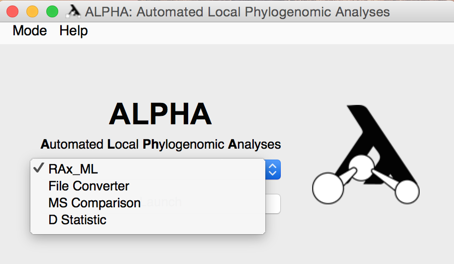
Once you enter any of these modes, you can use the "Mode" drop down menu in the upper left corner to enter a different one.

Here, we use the provided example files (see the folder "exampleFiles" in the ALPHA directory) to show how to use the software.
RAxML Mode
Run RAxML
For Standard Mode:
- Input the desired window size and offset, and select the desired model.
- If you select the Bootstrap option, input the desired confidence level and number of bootstraps to be run.
- To root the tree, select the Rooted option. Use the drop down menu to select the desired outgroup.
For Advanced Mode:
- If you select the Custom RAxML Command option, input your desired command without the -s and -n flags.
- To generate a species tree:
- If you select the Custom RAxML Command option, use the same parameters as above to input your command.
- To root your species tree, select the Rooted option and select your desired outgroup with the drop down menu on the right.
- Click the Generate button to create your species tree file.
In this example, we generate a species tree by running RAxML over the entire alignment, which does not require additional inputs.

After modifying these options to your preferences, click the Run RAxML button. The Generate Figures options will be available after you run RAxML.
Generate Figures
Select any number of the eight figures to generate. Aside from the informative sites heatmap RAxML must be run before generating these figures. Some of the figures require inputs in the Graph Options and Species Tree sections, so their necessary parameters are defined below:
For Top Topologies Tree Visualization, Windows to Top Topologies Scatter Plot, and Top Topologies Frequency Donut Plot:
- To ensure that the color coding for these visuals is correct, generate the three figures together.
- Input the number of most frequently occurring topologies that you want to generate figures for in the Number of Top Topologies section under Graph Options.
For Robinson-Foulds Distance Scatter Plot:
- Input the species tree by selecting a file or inputting a newick string under the Species Tree section. You can generate a species tree for this by following the steps in the Advanced mode of Run RAxML. It is not necessary that the species tree is rooted.
- If you select the Weighted option, ALPHA will generate the weighted Robinson-Foulds Distance Scatter Plot. Otherwise, it will generate both the weighted and unweighted graphs.
For p(GT|ST) Scatter Plot:
- Input the Input the species tree by selecting a file or inputting a newick string under the Species Tree section. You can generate a species tree for this by following the steps in the Advanced mode of Run RAxML. The tree must be rooted to generate this plot.
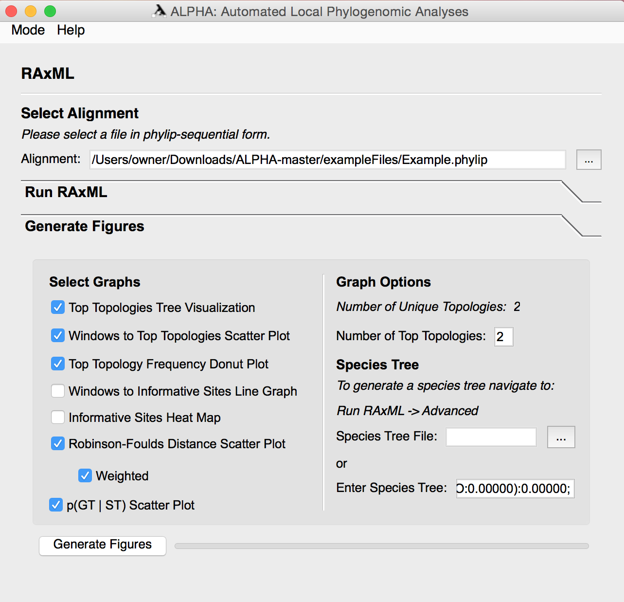
The informative sites heatmap provides a visualization of informative sites across an inputted alignment. Users can reduce the total number of sites that are used for the heatmap in order to speed up runs on extremely large files.
Once you have selected the desired figures to be generated, click the Generate Figures button.
To resize and manipulate the figures:
- All figures generated in ALPHA use a Matplotlib output interface, allowing users to customize figures to their liking. Hovering one’s cursor over the icons at the bottom of each figure’s output window provides a short description of each icon’s usage. The following describes each button from left to right.

- The home button reformats the plot to the default view.
- The left arrow button changes the plot to its previous view.
- The right arrow button changes the plot back to its former view if the previous view is selected.
- The arrow cross button allows users to change the view of the figure by panning across the plot.
- The magnifying glass button allows users to zoom to a rectangle on the plot.
- The sliders button allows users adjust the spacing and borders of their plots.
- The tight layout button gets rid of the border around the plot.
- The plot button allows users to customize the axes and curves of the figure.
- The axes tab allows users to change the min, max and scale of the axes, along with the title and axes labels. This tab also allows users to automatically generate a legend.
- The curves tab allows users to select each curve on the plot and alter its label, line style and color. Both the sliders button and plots button can be accessed by the “Configure Plot” menu at the top of the window; they can be found under “Configure Subplots” and “Configure Axis and Curves” respectively.
To save figures as images:
- The save button allows users to save and export the figure window to a specified location. This functionality can also be accessed under “Save As…” in the “File” menu at the top of the output window.
- All images can be exported to a desired save location, renamed and saved as one of the following file types: pdf, png, jpeg, tiff, svg, eps, rgba, pgf, and ps.
Walkthrough with Example File
Click the three dots on the line for alignment. This will bring up a file explorer in the ALPHA directory. From here choose the "exampleFiles" folder. In here you will find several files that are useful for learning about the usages of ALPHA. In this case select the "4TaxaExample.phylip" file. Before running RAxML you can generate a heatmap of the alignment's informative sites by clicking the checkbox next to "Informative Sites Heat Map" then clicking "Generate Figure". To run RAxML go to the "Run RAxML" tab here input a window size and offset. For this file we recommend 10000 and 10000. Click "Run RAxML" then go to the "Generate Figures" tab. Here you can select as many figures as you want then click "Generate Figures".
For more information on RAxML Mode and the figures it can generate, see the RAxML section above.
File Converter Mode
To use the file converter, first select the input file and its format. Then, specify the desired filename, location, and format of the output file. Click the convert button to create your new file.

For more information on the File Converter and its formats, see the File Converter section above.
MS Comparison Mode
First, select the MS Truth File that you want to analyze. Then, select either the Compare Against RAxML Directory option or the Compare Against MS File(s) option.
Compare Against RAxML Directory
To compare against a RAxML directory:
- Select the desired folder of RAxML files.
- Input the preferred window size and offset.
Compare Against MS File(s)
To select more than one MS file to compare against, simply click the + button to add the number of files you want to compare. Then, select one MS file per box. To remove a file, click the - button on the left side of the file input box. In the "exampleFiles" folder there are two files, "ExampleMS" and "ExampleMS2". New users can use these files to get a better understanding of the MS Comparison functionality.
Graphs
Select any number of the three graphs to generate them. Click the Compare button to run MS Comparison and generate the desired figures.
For more information on MS Comparison and the graphs it generates, see the MS Comparison section above.
D-statistic Mode
To compute the D-statistic, first input the desired alignment in phylip-sequential format.
Then, input the preferred window size and offset.
Using the provided four taxa tree, select your desired topology. Click the Run button to generate the D Statistic and the Windows to D-statistic Scatter Plot.
Users can subset from an alignment of more than 4 taxa. To get a better understanding of this use "6TaxaExample.txt" from the "exampleFiles" folder.
For more information on the D-statistic and what it outputs, see the D-statistic section above.
Developer Notes
For users looking to modify ALPHA source code we recommend using the PyCharm IDE with a Python 2.7.13 interpreter.
The user interface is created using PyQt4. More information on it can be found here: PyQt4. Individuals looking to alter the GUI must use the Qt Designer interface for the file "gui_layout.ui" located in the "module" folder. Alterations to the .ui file must be saved in the Qt Designer then pushed to the "gui_layout.py" file using the following command prompt command while in the "module" folder. If the command is not run then any changes made in the Qt Designer will not be updated properly.
```
pyuic4 gui_layout.ui -o gui_layout.py
```
All functions are executed within the "module" folder. Each of these files roughly corresponds to a different analysis function of ALPHA.
Plot outputs are each given their own window file where plot formatting and other aesthetics are dealt with. These files can be found in the "raxmlOutputWindows" folder and can be altered accordingly.
Add a New Page Walkthrough
1) Open Qt Designer this should have been installed along with PyQt and sip. A nice tutorial on the basics of Qt Designer as well as an alternative installation route via anaconda can be found at http://pythonforengineers.com/your-first-gui-app-with-python-and-pyqt/ 2) Click the file tab in the top left corner, click open and select the gui_layout.ui file in the Module folder of ALPHA 3) On the right in the object inspector the fourth tab is "stackedWidget" right click and click "insert page" choose the if you want the page to be before or after the current page Note: you can change the current page being edited using the left and right arrows on the top right corner of the ALPHA gui page 4) Scroll to the top of the widget box on the left side click and drag Vertical Layout onto the UI. Reposition and rescale as desired. 5) Scroll to the bottom of the widget box and find Label. Click and drag this into the box created by your vertical layout. 6) Double click TextLabel then type in "Hello World". To change the alignment of the text in the Property Editor section in the bottom right scroll down to QLabel. Click the arrow next to alignment next to Horizontal click AlignLeft then use the drop down menu to select the desired alignment type. 7) Click the Mode tab on the ALPHA interface then click Type Here and enter “Hello World” 8) While still selecting the text from step 8 got to the Property Editor in the bottom right corner and click the checkbox next to "checkable" 9) Use the arrows in the top right to ALPHA's home page. Double click the drop down menu. Then click the down arrow until the bottom selection is highlighted. Click the plus button and type in "Hello World". Save the ui file using the file tab.
Next we will alter ALPHA's python code to allow us to access the Hello World page using ALPHA's navigation bar.
10) Open command line, cd into the module folder in ALPHA. Then enter the command below. This pushes the changes from our PyQt ui file to the python file that main.py interacts with.
pyuic4 gui_layout.ui -o gui_layout.py11) Open main.py in a text editor or IDE (we recommend using PyCharm for this). Find the section of code that says "ADD NEW PAGE INFORMATION BELOW" (at the time of writing this was line 83). 12) Update the six dictionaries in this section of code by adding a comma then using the following code in order:
'inputPageHelloWorld': 6
'inputPageHelloWorld': {'x': 800, 'y': 900}
'inputPageHelloWorld': {'x': 450, 'y': 75}
'Hello World': 'inputPageHelloWorld,
'Hello World': self.actionHello_World
'inputPageHelloWorld': {'x': 600, 'y': 570}
13) Finally find the section of code with the header "CHANGE MODE" (at the time of writing this was line 141). Add the following line of code:
self.actionHello_World.triggered.connect(lambda: self.ensureSingleModeSelected(self.actionHello_World, 'inputPageHelloWorld'))Run main.py to and select Hello World from the menu to view your new page.
Tip: It is recommended developers rename widgets and page that they add in order to make variable names more informative. This can be done using the Object Inspector section in the top right corner of the page. Currently selected widgets will be highlighted in blue. Right click the desired widget then select Change Object Name.
Tip: If you add a widget at any point and it is initially too small to rescale using the cursor use the property editor in the bottom right corner of the screen.
Frequently Asked Questions
Q: Any click in a text box in the main window of the software leads to the following comment in the terminal: 2018-01-04 10:53:15.808 Python[89398:f07] unlockFocus called too many time. Is this an error?
A: No. This is currently a known issue with the PyQt GUI software. It is a harmless message without any effect on ALPHA and can safely be ignored.
Contributors
References
Cock PJA, Antao T, Chang JT, et al. Biopython: freely available Python tools for computational molecular biology and bioinformatics. Bioinformatics. 2009;25(11):1422-1423. doi:10.1093/bioinformatics/btp163.
Durand EY, Patterson N, Reich D, Slatkin M. Testing for Ancient Admixture between Closely Related Populations. Molecular Biology and Evolution. 2011;28(8):2239-2252. doi:10.1093/molbev/msr048.
ETE 3: Reconstruction, analysis and visualization of phylogenomic data. Jaime Huerta-Cepas, Francois Serra and Peer Bork. Mol Biol Evol 2016; doi: 10.1093/molbev/msw046
Green RE, Krause J, Briggs AW, et al. A Draft Sequence of the Neandertal Genome. Science (New York, NY). 2010;328(5979):710-722. doi:10.1126/science.1188021.
Richard R. Hudson; Generating samples under a Wright–Fisher neutral model of genetic variation. Bioinformatics 2002; 18 (2): 337-338. doi: 10.1093/bioinformatics/18.2.337
Hunter, John D. "Matplotlib: A 2D Graphics Environment." Computing in Science & Engineering 9.3 (2007): 90-95. 10.1109/MCSE.2007.55
Martin SH, Davey JW, Jiggins CD. Evaluating the Use of ABBA–BABA Statistics to Locate Introgressed Loci. Molecular Biology and Evolution. 2015;32(1):244-257. doi:10.1093/molbev/msu269.
Stamatakis A. 2014a. RAxML version 8: a tool for phylogenetic analysis and post-analysis of large phylogenies. Bioinformatics 30, 1312–1313. DOI: 10.1093/bioinformatics/btu033.
Stamatakis A. 2014b. The RAxML v8.0.X Manual
Sukumaran, J. and Mark T. Holder. 2010. DendroPy: A Python library for phylogenetic computing. Bioinformatics 26: 1569-1571.
Than C, Ruths D, Nakhleh L (2008) PhyloNet: a software package for analyzing and reconstructing reticulate evolutionary relationships. BMC Bioinformatics 9: 322
Yu Y, Degnan JH, Nakhleh L. The Probability of a Gene Tree Topology within a Phylogenetic Network with Applications to Hybridization Detection. Felsenstein J, ed. PLoS Genetics. 2012;8(4):e1002660. doi:10.1371/journal.pgen.1002660.