Purpose
Implementation of some known cellular automata. Use for academic purposes only.
Work in progress ...
Floor Field Model (cellular_automaton.py)
Reference
Cellular Automaton. Floor Field Model [Burstedde2001] Simulation of pedestriandynamics using a two-dimensional cellular automaton Physica A, 295, 507-525, 2001
Usage
python cellular_automaton.py <optional arguments>Optional arguments
| option | value | description |
|---|---|---|
-h, --help |
show this help message and exit | |
-s, --ks |
KS | sensitivity parameter for the Static Floor Field (default 2) |
-d, --kd |
KD | sensitivity parameter for the Dynamic Floor Field (default 1) |
-n, --numPeds |
NUMPEDS | Number of agents (default 10) |
-p, --plotS |
plot Static Floor Field | |
--plotD |
plot Dynamic Floor Field | |
--plotAvgD |
plot average Dynamic Floor Field | |
-P, --plotP |
plot Pedestrians | |
-r, --shuffle |
random shuffle | |
-v, --reverse |
reverse sequential update | |
-l, --log |
LOG | log file (default log.dat) |
--decay |
DECAY | the decay probability of the Dynamic Floor Field (default 0.2) |
--diffusion |
DIFFUSION | the diffusion probability of the Dynamic Floor Field (default 0.2) |
-W, --width |
WIDTH | the width of the simulation area in meter, excluding walls |
-H, --height |
HEIGHT | the height of the simulation room in meter, excluding walls |
-c, --clean |
remove files from directories dff/ sff/ and peds/ | |
-N, --nruns |
NRUNS | repeat the simulation N times (default 1) |
--parallel |
use multithreading | |
--moore |
use moore neighborhood (default Von Neumann) | |
--box |
from_x to_x from_y to_y | Rectangular box defined by 4 numbers, where agents will be distributed. (default the whole room) |
Simulation results
With the following parameter:
- Width of room: 30 m
- Hight of the room: 30 m
- Number of runs: 1
- Number of pedestrians 2000
- Diffusion parameter: 2
- Decay parameter: 0.2
- Static FF parameter: 2
- Dynamic FF parameter: 5
Call:
python cellular_automaton.py -W 30 -H 30 -N 1 -n 2000 --diffusion 2 --plotAvgD --plotD -d 5 -s 2 -P-
Video simulation
-
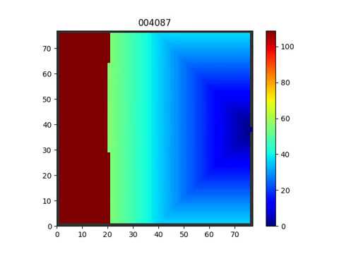
Dynamics floor field (averaged over time)

Comparison of different neighborhoods
Call the script with the option -moore to use the moore neighborhood. Otherwise, von Neumann neighborhood will be used as default.
The choice of the neighborhood has an influence on the evacuation time, as can seen below.

Moore neighborhood (video)
von Neumann neighborhood (video)

Todos:
todo: Different update schemes: sequential, shuffle sequential, reverse sequential.todo: visualisation of the cell states: (option-P)todo: make a video from the png's- todo: track cells with id for further trajectory analysis.
todo: implement the dynamic floor field- todo: implement the parallel update
- todo: implement the conflict friction
mu(in case of the parallel update) - todo: read geometry from a png file. See read_png.py.
ASEP model (asep_fast.py)
the Asymmetric Simple Exclusion Process (ASEP)
Reference
Rajewsky, N. and Santen, L. and Schadschneider, A. and Schreckenberg, M. The asymmetric exclusion process: Comparison of update procedures Journal of Statistical Physics, 1998
Usage
python asep_slow.py <optional arguments>Optional arguments
| option | value | descrption |
|---|---|---|
-h, --help |
show this help message and exit | |
-n, --np |
NUMPEDS | number of agents (default 10) |
-N, --nr |
NRUNS | number of runs (default 1) |
-m, --ms |
MS | max simulation steps (default 100) |
-w, --width |
WIDTH | width of the system (default 50) |
-p, --plotP |
plot Pedestrians | |
-r, --shuffle |
random shuffle | |
-v, --reverse |
reverse sequential update | |
-l, --log |
LOG | log file (default log.dat) |
Simulation results
the theoretical fundamental diagram can be reproduced, see figure. The size of the system should be reasonably high and the simulation time also.
Todos
- todo: implement TASEP
- todo: implement sequential update with all its variants.
- Remarque: There are two implementations of the asep. One it optimized using vector-operations from
numpy(asep_fast.py) and the other implementation is using explicit loops (asep_slow.py). The naming of the two variations is justified when measuring their execution time:python make_fd.py asep_fast.py: 0:56.71 real, 52.12 user, 4.03 sys python make_fd.py asep_slow.py: 1:15.42 real, 70.55 user, 4.23 sys