A book-style version of this primer is available at https://d-krupke.github.io/cpsat-primer/.
The CP-SAT Primer: Using and Understanding Google OR-Tools' CP-SAT Solver
By Dominik Krupke, TU Braunschweig
Many combinatorially difficult optimization problems can, despite their proven theoretical hardness, be solved reasonably well in practice. The most successful approach is to use Mixed Integer Linear Programming (MIP) to model the problem and then use a solver to find a solution. The most successful solvers for MIPs are, e.g., Gurobi and CPLEX, which are both commercial and expensive (though, free for academics). There are also some open source solvers, but they are often not as powerful as the commercial ones. However, even when investing in such a solver, the underlying techniques (Branch and Bound & Cut on Linear Relaxations) struggle with some optimization problems, especially if the problem contains a lot of logical constraints that a solution has to satisfy. In this case, the Constraint Programming (CP) approach may be more successful. For Constraint Programming, there are many open source solvers, but they usually do not scale as well as MIP-solvers and are worse in optimizing objective functions. While MIP-solvers are frequently able to optimize problems with hundreds of thousands of variables and constraints, the classical CP-solvers often struggle with problems with more than a few thousand variables and constraints. However, the relatively new CP-SAT of Google's OR-Tools suite shows to overcome many of the weaknesses and provides a viable alternative to MIP-solvers, being competitive for many problems and sometimes even superior.
Content
Whether you are from the MIP community seeking alternatives or CP-SAT is your first optimization solver, this book will guide you through the fundamentals of CP-SAT in the first part, demonstrating all its features. The second part will equip you with the skills needed to build and deploy optimization algorithms using CP-SAT.
The first part introduces the fundamentals of CP-SAT, starting with a chapter on installation. This chapter guides you through setting up CP-SAT and outlines the necessary hardware requirements. The next chapter provides a simple example of using CP-SAT, explaining the mathematical notation and its approximation in Python with overloaded operators. You will then progress to basic modeling, learning how to create variables, objectives, and fundamental constraints in CP-SAT.
Following this, a chapter on advanced modeling will teach you how to handle complex constraints, such as circuit constraints and intervals, with practical examples. Another chapter discusses specifying CP-SAT's behavior, including setting time limits and using parallelization. You will also find a chapter on interpreting CP-SAT logs, which helps you understand how well CP-SAT is managing your problem. Additionally, there is an overview of the underlying techniques used in CP-SAT. The first part concludes with a chapter comparing CP-SAT with other optimization techniques and tools, providing a broader context.
The second part delves into more advanced topics, focusing on general skills like coding patterns and benchmarking rather than specific CP-SAT features. A chapter on coding patterns offers basic design patterns for creating maintainable algorithms with CP-SAT. Another chapter explains how to provide your optimization algorithm as a service by building an optimization API. There is also a chapter on developing powerful heuristics using CP-SAT for particularly difficult or large problems. The second part concludes with a chapter on benchmarking, offering guidance on how to scientifically benchmark your model and interpret the results.
Target Audience
I wrote this book for my computer science students at TU Braunschweig, and it is used as supplementary material in my algorithm engineering courses. Initially, we focused on Mixed Integer Programming (MIP), with CP-SAT discussed as an alternative. However, we recently began using CP-SAT as the first optimization solver due to its high-level interface, which is much easier for beginners to grasp. Despite this shift, because MIP is more commonly used, the book includes numerous comparisons to MIP. Thus, it is designed to be beginner-friendly while also addressing the needs of MIP users seeking alternatives.
Unlike other books aimed at mathematical optimization or operations research students, this one, aimed at computer science students, emphasizes coding over mathematics or business cases, providing a hands-on approach to learning optimization. The second part of the book can also be interesting for more advanced users, providing content that I found missing in other books on optimization.
Table of Content
Part 1: The Basics
- Installation: Quick installation guide.
- Example: A short example, showing the usage of CP-SAT.
- Basic Modeling: An overview of variables, objectives, and constraints.
- Advanced Modeling: More complex constraints, such as circuit constraints and intervals.
- Parameters: How to specify CP-SATs behavior, if needed. Timelimits, hints, assumptions, parallelization, ...
- Understanding the Log: How to interpret the log
- How does it work?: After we know what we can do with CP-SAT, we look into how CP-SAT will do all these things.
- Alternatives: An overview of the different optimization techniques and tools available. Putting CP-SAT into context.
Part 2: Advanced Topics
- Coding Patterns: Basic design patterns for creating maintainable algorithms.
- (DRAFT) Building an Optimization API How to build a scalable API for long running optimization jobs.
- Large Neighborhood Search: The use of CP-SAT to create more powerful heuristics.
- Benchmarking your Model: How to benchmark your model and how to interpret the results.
Background
This book assumes you are fluent in Python, and have already been introduced to combinatorial optimization problems. In case you are just getting into combinatorial optimization and are learning on your own, I recommend starting with the free Coursera course, Discrete Optimization, taught by Pascal Van Hentenryck and Carleton Coffrin. This course provides a comprehensive introduction in a concise format.
For an engaging exploration of a classic problem within this domain, In Pursuit of the Traveling Salesman by Bill Cook is highly recommended. This book, along with this YouTube talk by the author that lasts about an hour, offers a practical case study of the well-known Traveling Salesman Problem. It not only introduces fundamental techniques but also delves into the community and historical context of the field.
Additionally, the article Mathematical Programming by CP-SAT's competitor Gurobi offers an insightful introduction to mathematical programming and modeling. In this context, the term "Programming" does not refer to coding; rather, it originates from an earlier usage of the word "program", which denoted a plan of action or a schedule. If this distinction is new to you, it is a strong indication that you would benefit from reading this article.
About the Main Author: Dr. Dominik Krupke is a postdoctoral researcher with the Algorithms Division at TU Braunschweig. He specializes in practical solutions to NP-hard problems. Initially focused on theoretical computer science, he now applies his expertise to solve what was once deemed impossible, frequently with the help of CP-SAT. This primer on CP-SAT, first developed as course material for his students, has been extended in his spare time to cater to a wider audience.
Found a mistake? Please open an issue or a pull request. You can also just write me a quick mail to
krupked@gmail.com.Want to contribute? If you are interested in contributing, please open an issue or email me with a brief description of your proposal. We can then discuss the details. I welcome all assistance and am open to expanding the content. Contributors to any section or similar input will be recognized as coauthors.
Want to use/share this content? This tutorial can be freely used under CC-BY 4.0. Smaller parts can even be copied without any acknowledgement for non-commercial, educational purposes.
Part 1: The Basics
Installation
We are using Python 3 in this primer and assume that you have a working Python 3 installation as well as the basic knowledge to use it. There are also interfaces for other languages, but Python 3 is, in my opinion, the most convenient one, as the mathematical expressions in Python are very close to the mathematical notation (allowing you to spot mathematical errors much faster). Only for huge models, you may need to use a compiled language such as C++ due to performance issues. For smaller models, you will not notice any performance difference.
The installation of CP-SAT, which is part of the OR-Tools package, is very easy and can be done via Python's package manager pip.
pip3 install -U ortoolsThis command will also update an existing installation of OR-Tools. As this tool is in active development, it is recommended to update it frequently. We actually encountered wrong behavior, i.e., bugs, in earlier versions that then have been fixed by updates (this was on some more advanced features, do not worry about correctness with basic usage).
I personally like to use Jupyter Notebooks for experimenting with CP-SAT.
What hardware do you need?
It is important to note that for CP-SAT usage, you do not need the capabilities of a supercomputer. A standard laptop is often sufficient for solving many problems. The primary requirements are CPU power and memory bandwidth, with a GPU being unnecessary.
In terms of CPU power, the key is balancing the number of cores with the performance of each individual core. CP-SAT leverages all available cores, implementing different strategies on each. Depending on the number of cores, CP-SAT will behave differently. However, the effectiveness of these strategies can vary, and it is usually not apparent which one will be most effective. A higher single-core performance means that your primary strategy will operate more swiftly. I recommend a minimum of 4 cores and 16GB of RAM.
While CP-SAT is quite efficient in terms of memory usage, the amount of available memory can still be a limiting factor in the size of problems you can tackle. When it came to setting up our lab for extensive benchmarking at TU Braunschweig, we faced a choice between desktop machines and more expensive workstations or servers. We chose desktop machines equipped with AMD Ryzen 9 7900 CPUs (Intel would be equally suitable) and 96GB of DDR5 RAM, managed using Slurm. This decision was driven by the fact that the performance gains from higher-priced workstations or servers were relatively marginal compared to their significantly higher costs. When on the road, I am often still able to do stuff with my old Intel Macbook Pro from 2018 with an i7 and only 16GB of RAM, but large models will overwhelm it. My workstation at home with AMD Ryzen 7 5700X and 32GB of RAM on the other hand rarely has any problems with the models I am working on.
For further guidance, consider the hardware recommendations for the Gurobi solver, which are likely to be similar. Since we frequently use Gurobi in addition to CP-SAT, our hardware choices were also influenced by their recommendations.
A Simple Example
Before we dive into any internals, let us take a quick look at a simple application of CP-SAT. This example is so simple that you could solve it by hand, but know that CP-SAT would (probably) be fine with you adding a thousand (maybe even ten- or hundred-thousand) variables and constraints more. The basic idea of using CP-SAT is, analogous to MIPs, to define an optimization problem in terms of variables, constraints, and objective function, and then let the solver find a solution for it. We call such a formulation that can be understood by the corresponding solver a model for the problem. For people not familiar with this declarative approach, you can compare it to SQL, where you also just state what data you want, not how to get it. However, it is not purely declarative, because it can still make a huge(!) difference how you model the problem and getting that right takes some experience and understanding of the internals. You can still get lucky for smaller problems (let us say a few hundred to thousands of variables) and obtain optimal solutions without having an idea of what is going on. The solvers can handle more and more 'bad' problem models effectively with every year.
[!NOTE]
A model in mathematical programming refers to a mathematical description of a problem, consisting of variables, constraints, and optionally an objective function that can be understood by the corresponding solver class. Modelling refers to transforming a problem (instance) into the corresponding framework, e.g., by making all constraints linear as required for Mixed Integer Linear Programming. Be aware that the SAT-community uses the term model to refer to a (feasible) variable assignment, i.e., solution of a SAT-formula. If you struggle with this terminology, maybe you want to read this short guide on Math Programming Modelling Basics.
Our first problem has no deeper meaning, except for showing the basic workflow of creating the variables (x and y), adding the constraint $x+y<=30$ on them, setting the objective function (maximize $30x + 50y$), and obtaining a solution:
from ortools.sat.python import cp_model

model = cp_model.CpModel()

# Variables
x = model.new_int_var(0, 100, "x")
y = model.new_int_var(0, 100, "y")

# Constraints
model.add(x + y <= 30)

# Objective
model.maximize(30 * x + 50 * y)

# Solve
solver = cp_model.CpSolver()
status = solver.solve(model)

# The status tells us if we were able to compute an optimal solution.
assert status == cp_model.OPTIMAL, "Could not find optimal solution."

# Print the optimal solution.
print(f"x={solver.value(x)},  y={solver.value(y)}")
x=0, y=30Pretty easy, right? For solving a generic problem, not just one specific
instance, you would of course create a dictionary or list of variables and use
something like model.add(sum(vars)<=n), because you do not want to create the
model by hand for larger instances.
[!TIP]
The solver can return five different statuses:
Status Code Description UNKNOWN0 The solver has not yet run. MODEL_INVALID1 The model is invalid. You will rarely see that status. FEASIBLE2 The model has a feasible, but not necessarily optimal, solution. If your model does not have an objective, every feasible model will return OPTIMAL, which may be counterintuitive.INFEASIBLE3 The model has no feasible solution. This means that your constraints are too restrictive. OPTIMAL4 The model has an optimal solution. If your model does not have an objective, OPTIMALis returned instead ofFEASIBLE.The status
UNBOUNDEDdoes not exist, as CP-SAT does not have unbounded variables.
For larger models, CP-SAT will unfortunately not always able to compute an optimal solution. However, the good news is that the solver will likely still find a satisfactory solution and provide a bound on the optimal solution. Once you reach this point, understanding how to interpret the solver's log becomes crucial for analyzing the solver's performance. We will learn more about this later.
Mathematical Model
The mathematical model of the code above would usually be written by experts something like this:
\max 30x + 50y\text{s.t. } x+y \leq 30\quad 0\leq x \leq 100\quad 0\leq y \leq 100x,y \in \mathbb{Z}The s.t. stands for subject to, sometimes also read as such that.
Overloading
One aspect of using CP-SAT solver that often poses challenges for learners is
understanding operator overloading in Python and the distinction between the two
types of variables involved. In this context, x and y serve as mathematical
variables. That is, they are placeholders that will only be assigned specific
values during the solving phase. To illustrate this more clearly, let us explore
an example within the Python shell:
>>> model = cp_model.CpModel()
>>> x = model.new_int_var(0, 100, "x")
>>> x
x(0..100)
>>> type(x)
<class 'ortools.sat.python.cp_model.IntVar'>
>>> x + 1
sum(x(0..100), 1)
>>> x + 1 <= 1
<ortools.sat.python.cp_model.BoundedLinearExpression object at 0x7d8d5a765df0>
In this example, x is not a conventional number but a placeholder defined to
potentially assume any value between 0 and 100. When 1 is added to x, the
result is a new placeholder representing the sum of x and 1. Similarly,
comparing this sum to 1 produces another placeholder, which encapsulates the
comparison of the sum with 1. These placeholders do not hold concrete values at
this stage but are essential for defining constraints within the model.
Attempting operations like if x + 1 <= 1: print("True") will trigger a
NotImplementedError, as the condition x+1<=1 cannot be evaluated directly.
Although this approach to defining models might initially seem perplexing, it facilitates a closer alignment with mathematical notation, which in turn can make it easier to identify and correct errors in the modeling process.
More examples
If you are not yet satisfied, this folder contains many Jupyter Notebooks with examples from the developers. For example
- multiple_knapsack_sat.ipynb shows how to solve a multiple knapsack problem.
- nurses_sat.ipynb shows how to schedule the shifts of nurses.
- bin_packing_sat.ipynb shows how to solve a bin packing problem.
- ... (if you know more good examples I should mention here, please let me know!)
Further, you can find an extensive and beginner-friendly example on scheduling workers here.
Now that you have seen a minimal model, let us explore the various options available for problem modeling. While an experienced optimizer might be able to handle most problems using just the elements previously discussed, clearly expressing your intentions can help CP-SAT optimize your problem more effectively.
Basic Modeling
In this chapter, we dive into the basic modeling capabilities of CP-SAT. CP-SAT
provides an extensive set of constraints, closer to high-level modeling
languages like MiniZinc than to traditional Mixed Integer Programming (MIP). For
example, it offers constraints like all_different and
add_multiplication_equality. These advanced features reduce the need for
modeling complex logic strictly through linear constraints, though they also
increase the interface's complexity. However, not all constraints are equally
efficient; linear and boolean constraints are generally most efficient, whereas
constraints like add_multiplication_equality can be significantly more
resource-intensive.
[!TIP]
If you are transitioning from Mixed Integer Programming (MIP), you might be used to manually implementing higher-level constraints and optimizing Big-M parameters for better performance. With CP-SAT, such manual adjustments are generally unnecessary. CP-SAT operates differently from typical MIP solvers by relying less on linear relaxation and more on its underlying SAT-solver and propagators to efficiently manage logical constraints. Embrace the higher-level constraints—they are often more efficient in CP-SAT.
This primer has been expanded to cover all constraints across two chapters, complete with various examples to illustrate the contexts in which they can be used. However, mastering modeling involves much more than just an understanding of constraints. It requires a deep appreciation of the principles and techniques that make models effective and applicable to real-world problems.
For a more detailed exploration of modeling, consider "Model Building in Mathematical Programming" by H. Paul Williams, which offers extensive insight into the subject, including practical applications. While this book is not specific to CP-SAT, the foundational techniques and concepts are broadly applicable. Additionally, for those new to this area or transitioning from MIP solutions, studying Gurobi's modeling approach through this video course might prove helpful. While many principles overlap, some strategies unique to CP-SAT can better address cases where traditional MIP-solvers struggle.
Additional resources on mathematical modeling (not CP-SAT specific):
- Math Programming Modeling Basics by Gurobi: This resource provides a solid introduction to the basics of mathematical modeling.
- Modeling with Gurobi Python: A comprehensive video course on modeling with Gurobi, highlighting concepts that are also applicable to CP-SAT.
- Model Building in Mathematical Programming by H. Paul Williams: An extensive guide to mathematical modeling techniques.
Elements:
- Variables:
new_int_var,new_bool_var,new_constant,new_int_var_series,new_bool_var_series- Domain Variables:
new_int_var_from_domain
- Domain Variables:
- Objectives:
minimize,maximize - Linear Constraints:
add,add_linear_constraint - Logical Constraints (Propositional Logic):
add_implication,add_bool_or,add_at_least_one,add_at_most_one,add_exactly_one,add_bool_and,add_bool_xor - Conditional Constraints (Reification):
only_enforce_if - Absolute Values and Max/Min:
add_min_equality,add_max_equality,add_abs_equality - Multiplication, Division, and Modulo:
add_modulo_equality,add_multiplication_equality,add_division_equality - All Different:
add_all_different - Domains and Combinations:
add_allowed_assignments,add_forbidden_assignments - Array/Element Constraints:
add_element,add_inverse
The more advanced constraints add_circuit, add_multiple_circuit,
add_automaton,add_reservoir_constraint,
add_reservoir_constraint_with_active, new_interval_var,
new_interval_var_series, new_fixed_size_interval_var,
new_optional_interval_var, new_optional_interval_var_series,
new_optional_fixed_size_interval_var,
new_optional_fixed_size_interval_var_series, add_no_overlap,
add_no_overlap_2d, and add_cumulative are discussed in the next chapter.
Variables
There are two important types of variables in CP-SAT: Booleans and Integers (which are actually converted to Booleans, but more on this later). There are also, e.g., interval variables, but they are actually rather a combination of integral variables and discussed later. For the integer variables, you have to specify a lower and an upper bound.
model = cp_model.CpModel()

# Integer variable z with bounds -100 <= z <= 100
z = model.new_int_var(-100, 100, "z")  # new syntax
z_ = model.NewIntVar(-100, 100, "z_")  # old syntax

# Boolean variable b
b = model.new_bool_var("b")  # new syntax
b_ = model.NewBoolVar("b_")  # old syntax

# Implicitly available negation of b:
not_b = ~b  # will be 1 if b is 0 and 0 if b is 1
not_b_ = b.Not()  # old syntax
Additionally, you can use model.new_int_var_series and
model.new_bool_var_series to create multiple variables at once from a pandas
Index. This is especially useful if your data is given in a pandas DataFrame.
However, there is no performance benefit in using this method, it is just more
convenient.
model = cp_model.CpModel()

# Create an Index from 0 to 9
index = pd.Index(range(10), name="index")

# Create a pandas Series with 10 integer variables matching the index
xs = model.new_int_var_series("x", index, 0, 100)

# List of boolean variables
df = pd.DataFrame(
    data={"weight": [1 for _ in range(10)], "value": [3 for _ in range(10)]},
    index=["A", "B", "C", "D", "E", "F", "G", "H", "I", "J"],
)
bs = model.new_bool_var_series("b", df.index)  # noqa: F841

# Using the dot product on the pandas DataFrame is actually a pretty
# convenient way to create common linear expressions.
model.add(bs @ df["weight"] <= 100)
model.maximize(bs @ df["value"])
Additionally, there is the new_constant-method, which allows you to create a
variable that is constant. I have not found a use case for this yet, let me know
if you have one.
[!TIP]
In an older project, I observed that maintaining tight bounds on integer variables can significantly impact performance. Employing a heuristic to find a reasonable initial solution, which then allowed for tighter bounds, proved worthwhile, even though the bounds were just a few percent tighter. Although this project was several years ago and CP-SAT has advanced considerably since then, I still recommend keeping the bounds on the variables' ranges as tight as possible.
There are no continuous/floating point variables (or even constants) in CP-SAT: If you need floating point numbers, you have to approximate them with integers by some resolution. For example, you could simply multiply all values by 100 for a step size of 0.01. A value of 2.35 would then be represented by 235. This could probably be implemented in CP-SAT directly, but doing it explicitly is not difficult, and it has numerical implications that you should be aware of.
The absence of continuous variables may appear as a substantial limitation, especially for those with a background in linear optimization where continuous variables are typically regarded as the simpler component. However, if your problem includes only a few continuous variables that must be approximated using large integers and involves complex constraints such as absolute values, while the majority of the problem is dominated by logical constraints, CP-SAT can often outperform mixed-integer programming solvers. It is only when a problem contains a substantial number of continuous variables and benefits significantly from strong linear relaxation that mixed-integer programming solvers will have a distinct advantage, despite CP-SAT having a propagator based on the dual simplex method.
I analyzed the impact of resolution (i.e., the factor by which floating point numbers are multiplied) on the runtime of CP-SAT, finding that the effect varied depending on the problem. For one problem, the runtime increased only logarithmically with the resolution, allowing the use of a very high resolution of 100,000x without significant issues. In contrast, for another problem, the runtime increased roughly linearly with the resolution, making high resolutions impractical. The runtime for different factors in this case was: 1x: 0.02s, 10x: 0.7s, 100x: 7.6s, 1000x: 75s, and 10,000x: over 15 minutes, even though the solution remained the same, merely scaled. Therefore, while high resolutions may be feasible for some problems using CP-SAT, it is essential to verify their influence on runtime, as the impact can be considerable.
In my experience, boolean variables are crucial in many combinatorial optimization problems. For instance, the famous Traveling Salesman Problem consists solely of boolean variables. Therefore, implementing a solver that specializes in boolean variables using a SAT-solver as a foundation, such as CP-SAT, is a sensible approach. CP-SAT leverages the strengths of SAT-solving techniques, which are highly effective for problems dominated by boolean variables.
You may wonder why it is necessary to explicitly name the variables in CP-SAT. While there does not appear to be a technical reason for this requirement, naming the variables can be extremely helpful for debugging purposes. Understanding the naming scheme of the variables allows you to more easily interpret the internal representation of the model, facilitating the identification and resolution of issues. To be fair, there have only been a few times when I actually needed to take a closer at the internal representation, and in most of the cases I would have preferred not to have to name the variables.
Domain Variables
When dealing with integer variables that you know will only need to take certain values, or when you wish to limit their possible values, domain variables can become interesting. Unlike regular integer variables, domain variables are tailored to represent a specific set of values. This approach can enhance efficiency when the domain - the range of sensible values - is small. However, it may not be the best choice for larger domains.
CP-SAT works by converting all integer variables into boolean variables (warning: simplification). For each potential value, it creates two boolean variables: one indicating whether the integer variable is equal to this value, and another indicating whether it is less than or equal to it. This is called an order encoding. At first glance, this might suggest that using domain variables is always preferable, as it appears to reduce the number of boolean variables needed.
However, CP-SAT employs a lazy creation strategy for these boolean variables. This means it only generates them as needed, based on the solver's decision-making process. Therefore, an integer variable with a wide range - say, from 0 to 100 - will not immediately result in 200 boolean variables. It might lead to the creation of only a few, depending on the solver's requirements.
Limiting the domain of a variable can have drawbacks. Firstly, defining a domain explicitly can be computationally costly and increase the model size drastically as it now need to contain not just a lower and upper bound for a variable but an explicit list of numbers (model size is often a limiting factor). Secondly, by narrowing down the solution space, you might inadvertently make it more challenging for the solver to find a viable solution. First, try to let CP-SAT handle the domain of your variables itself and only intervene if you have a good reason to do so.
If you choose to utilize domain variables for their benefits in specific scenarios, here is how to define them:
from ortools.sat.python import cp_model

model = cp_model.CpModel()

# Define a domain with selected values
domain = cp_model.Domain.from_values([2, 5, 8, 10, 20, 50, 90])

# Can also be done via intervals
domain_2 = cp_model.Domain.from_intervals([[8, 12], [14, 20]])

# There are also some operations available
domain_3 = domain.union_with(domain_2)

# Create a domain variable within this defined domain
x = model.new_int_var_from_domain(domain, "x")
This example illustrates the process of creating a domain variable x that can
only take on the values specified in domain. This method is particularly
useful when you are working with variables that only have a meaningful range of
possible values within your problem's context.
Objectives
Not every problem necessitates an objective; sometimes, finding a feasible solution is sufficient. CP-SAT excels at finding feasible solutions, a task at which mixed-integer programming (MIP) solvers often do not perform as well. However, CP-SAT is also capable of effective optimization, which is an area where older constraint programming solvers may lag, based on my experience.
CP-SAT allows for the minimization or maximization of a linear expression. You
can model more complex expressions by using auxiliary variables and additional
constraints. To specify an objective function, you can use the model.minimize
or model.maximize commands with a linear expression. This flexibility makes
CP-SAT a robust tool for a variety of optimization tasks.
# Basic model with variables and constraints
model = cp_model.CpModel()
x = model.new_int_var(-100, 100, "x")
y = model.new_int_var(-100, 100, "y")
model.add(x + 10 * y <= 100)

# Minimize 30x + 50y
model.maximize(30 * x + 50 * y)
Let us look on how to model more complicated expressions, using boolean variables and generators.
model = cp_model.CpModel()
x_vars = [model.new_bool_var(f"x{i}") for i in range(10)]
model.minimize(
    sum(i * x_vars[i] if i % 2 == 0 else i * x_vars[i].Not() for i in range(10))
)
This objective evaluates to
\min \sum_{i=0}^{9} i\cdot x_i \text{ if } i \text{ is even else } i\cdot \neg x_iTo implement a lexicographic optimization, you can do multiple rounds and always fix the previous objective as constraint.
# some basic model
model = cp_model.CpModel()
x = model.new_int_var(-100, 100, "x")
y = model.new_int_var(-100, 100, "y")
z = model.new_int_var(-100, 100, "z")
model.add(x + 10 * y - 2 * z <= 100)

# Define the objectives
first_objective = 30 * x + 50 * y
second_objective = 10 * x + 20 * y + 30 * z

# Optimize for the first objective
model.maximize(first_objective)
solver = cp_model.CpSolver()
solver.solve(model)

# Fix the first objective and optimize for the second
model.add(first_objective == int(solver.objective_value))  # fix previous objective
model.minimize(second_objective)  # optimize for second objective
solver.solve(model)
To handle non-linear objectives in CP-SAT, you can employ auxiliary variables
and constraints. For instance, to incorporate the absolute value of a variable
into your objective, you first create a new variable representing this absolute
value. Shortly, you will learn more about setting up these types of constraints.
Below is a Python example demonstrating how to model and minimize the absolute
value of a variable x:
# Assuming x is already defined in your model
abs_x = model.new_int_var(
    0, 100, "|x|"
)  # Create a variable to represent the absolute value of x
model.add_abs_equality(target=abs_x, expr=x)  # Define abs_x as the absolute value of x
model.minimize(abs_x)  # Set the objective to minimize abs_x
The constraints available to define your feasible solution space will be discussed in the following section.
Linear Constraints
These are the classical constraints also used in linear optimization. Remember that you are still not allowed to use floating point numbers within it. Same as for linear optimization: You are not allowed to multiply a variable with anything else than a constant and also not to apply any further mathematical operations.
model.add(10 * x + 15 * y <= 10)
model.add(x + z == 2 * y)

# This one actually is not linear but still works.
model.add(x + y != z)

# Because we are working on integers, the true smaller or greater constraints
# are trivial to implement as x < z is equivalent to x <= z-1
model.add(x < y + z)
model.add(y > 300 - 4 * z)
Note that != can be slower than the other (<=, >=, ==) constraints,
because it is not a linear constraint. If you have a set of mutually !=
variables, it is better to use all_different (see below) than to use the
explicit != constraints.
[!WARNING]
If you use intersecting linear constraints, you may get problems because the intersection point needs to be integral. There is no such thing as a feasibility tolerance as in Mixed Integer Programming-solvers, where small deviations are allowed. The feasibility tolerance in MIP-solvers allows, e.g., 0.763445 == 0.763439 to still be considered equal to counter numerical issues of floating point arithmetic. In CP-SAT, you have to make sure that values can match exactly.
Let us look at the following example with two linear equality constraints:
x - y = 04-y = 2yx, y \geq 0You can verify that $x=4/3$ and $y=4/3$ is a feasible solution. However, coding this in CP-SAT results in an infeasible solution:
model = cp_model.CpModel()
x = model.new_int_var(-100, 100, "x")
y = model.new_int_var(-100, 100, "y")

model.add(x - y == 0)
model.add(4 - x == 2 * y)

solver = cp_model.CpSolver()
status = solver.solve(model)
assert status == cp_model.INFEASIBLE
Even using scaling techniques, such as multiplying integer variables by 1,000,000 to increase the resolution, would not render the model feasible. While common linear programming solvers would handle this model without issue, CP-SAT struggles unless modifications are made to eliminate fractions, such as multiplying all terms by 3. However, this requires manual intervention, which undermines the idea of using a solver. These limitations are important to consider, although such scenarios are rare in practical applications.
If you have a lower and an upper bound for a linear expression, you can also use
the add_linear_constraint-method, which allows you to specify both bounds in
one go.
model.add_linear_constraint(linear_expr=10 * x + 15 * y, lb=-100, ub=10)The similar sounding AddLinearExpressionInDomain is discussed later.
Logical Constraints (Propositional Logic)
Propositional logic allows us to describe relationships between true or false statements using logical operators. Consider a simple scenario where we define three Boolean variables:
b1 = model.new_bool_var("b1")
b2 = model.new_bool_var("b2")
b3 = model.new_bool_var("b3")
These variables, b1, b2, and b3, represent distinct propositions whose
truth values are to be determined by the model.
You can obtain the negation of a Boolean variable by using ~ or the
.Not()-method. The resulting variable can be used just like the original
variable:
not_b1 = ~b1  # Negation of b1
not_b2 = b2.Not()  # Alternative notation for negation
Note that you can use more than three variables in all of the following
examples, except for add_implication which is only defined for two variables.
[!WARNING]
Boolean variables are essentially special integer variables restricted to the domain of 0 and 1. Therefore, you can incorporate them into linear constraints as well. However, it is important to note that integer variables, unlike Boolean variables, cannot be used in Boolean constraints. This is a distinction from some programming languages, like Python, where integers can sometimes substitute for Booleans.
Adding Logical OR Constraints
The logical OR operation ensures that at least one of the specified conditions holds true. To model this, you can use:
model.add_bool_or(b1, b2, b3)  # b1 or b2 or b3 must be true
model.add_at_least_one([b1, b2, b3])  # Alternative notation
model.add(b1 + b2 + b3 >= 1)  # Alternative linear notation using '+' for OR
Both lines ensure that at least one of b1, b2, or b3 is true.
Adding Logical AND Constraints
The logical AND operation specifies that all conditions must be true
simultaneously. To model conditions where b1 is true and both b2 and b3
are false, you can use:
model.add_bool_and(b1, b2.Not(), b3.Not())  # b1 and not b2 and not b3 must all be true
model.add_bool_and(b1, ~b2, ~b3)  # Alternative notation using '~' for negation
The add_bool_and method is most effective when used with the only_enforce_if
method. For cases not utilizing only_enforce_if a simple AND-clause such as
$\left( b_1 \land \neg b_2 \land \neg b_3 \right)$ becomes redundant by simply
substituting $b_1$ with 1 and $b_2, b_3$ with 0. In straightforward
scenarios, consider substituting these variables with their constant values to
reduce unnecessary complexity, especially in larger models where size and
manageability are concerns. In smaller or simpler models, CP-SAT efficiently
handles these redundancies, allowing you to focus on maintaining clarity and
readability in your model.
Adding Logical XOR Constraints
The logical XOR (exclusive OR) operation ensures that an odd number of operands are true. It is crucial to understand this definition, as it has specific implications when applied to more than two variables:
- For two variables, such as
b1 XOR b2, the operation returns true if exactly one of these variables is true, which aligns with the "exactly one" constraint for this specific case. - For three or more variables, such as in the expression
b1 XOR b2 XOR b3, the operation returns true if an odd number of these variables are true. This includes scenarios where one or three variables are true, assuming the total number of variables involved is three.
This characteristic of XOR can be somewhat complex but is crucial for modeling scenarios where the number of true conditions needs to be odd:
model.add_bool_xor(b1, b2)  # Returns true if exactly one of b1 or b2 is true
model.add_bool_xor(
    b1, b2, b3
)  # Returns true if an odd number of b1, b2, b3 are true (i.e., one or three)
Specifying Unique Conditions
To enforce that exactly one or at most one of the variables is true, use:
model.add_exactly_one([b1, b2, b3])  # Exactly one of the variables must be true
model.add_at_most_one([b1, b2, b3])  # No more than one of the variables should be true
These constraints are useful for scenarios where exclusive choices must be modeled.
You could alternatively also use add.
model.add(b1 + b2 + b3 == 1)  # Exactly one of the variables must be true
model.add(b1 + b2 + b3 <= 1)  # No more than one of the variables should be true
Modeling Implications
Logical implication, denoted as ->, indicates that if the first condition is
true, the second must also be true. This can be modeled as:
model.add_implication(b1, b2) # If b1 is true, then b2 must also be trueYou could also use add.
model.add(b2 >= b1) # If b1 is true, then b2 must also be trueConditional Constraints (Reification)
In practical applications, scenarios often arise where conditions dictate the enforcement of certain constraints. For instance, "if this condition is true, then a specific constraint should apply," or "if a constraint is violated, a penalty variable is set to true, triggering another constraint." Additionally, real-world constraints can sometimes be bypassed with financial or other types of concessions, such as renting a more expensive truck to exceed a load limit, or allowing a worker to take a day off after a double shift.
In constraint programming, reification involves associating a Boolean variable with a constraint to capture its truth value, thereby turning the satisfaction of the constraint into a variable that can be used in further constraints. Full reification links a Boolean variable such that it is
Trueif the constraint is satisfied andFalseotherwise, enabling the variable to be directly used in other decisions or constraints. Conversely, half-reification, or implied constraints, involves a one-way linkage where the Boolean variable beingTrueimplies the constraint must be satisfied, but its beingFalsedoes not necessarily indicate anything about the constraint's satisfaction. This approach is particularly useful for expressing complex conditional logic and for modeling scenarios where only the satisfaction, and not the violation, of a constraint needs to be explicitly handled.
To effectively manage these conditional scenarios, CP-SAT offers the
only_enforce_if-method for linear and some Boolean constraints, which
activates a constraint only if a specified condition is met. This method is not
only typically more efficient than traditional methods like the
Big-M method but also simplifies
the model by eliminating the need to determine an appropriate Big-M value.
# A value representing the load that needs to be transported
load_value = model.new_int_var(0, 100, "load_value")

# ... some logic to determine the load value ...

# A variable to decide which truck to rent
truck_a = model.new_bool_var("truck_a")
truck_b = model.new_bool_var("truck_b")
truck_c = model.new_bool_var("truck_c")

# Only rent one truck
model.add_at_most_one([truck_a, truck_b, truck_c])

# Depending on which truck is rented, the load value is limited
model.add(load_value <= 50).only_enforce_if(truck_a)
model.add(load_value <= 80).only_enforce_if(truck_b)
model.add(load_value <= 100).only_enforce_if(truck_c)

# Some additional logic
driver_has_big_truck_license = model.new_bool_var("driver_has_big_truck_license")
driver_has_special_license = model.new_bool_var("driver_has_special_license")
# Only drivers with a big truck license or a special license can rent truck c
model.add_bool_or(
    driver_has_big_truck_license, driver_has_special_license
).only_enforce_if(truck_c)

# Minimize the rent cost
model.minimize(30 * truck_a + 40 * truck_b + 80 * truck_c)
You can also use negations in the only_enforce_if method.
model.add(x + y == 10).only_enforce_if(~b1)You can also pass a list of Boolean variables to only_enforce_if, in which
case the constraint is only enforced if all of the variables in the list are
true.
model.add(x + y == 10).only_enforce_if([b1, ~b2]) # only enforce if b1 AND NOT b2[!WARNING]
While
only_enforce_ifin CP-SAT is often more efficient than similar concepts in classical MIP-solvers, it can still impact the performance of CP-SAT significantly. Doing some additional reasoning, you can often find a more efficient way to model your problem without having to useonly_enforce_if. For logical constraints, there are actually straight-forward methods in propositional calculus. Asonly_enforce_ifis often a more natural way to model your problem, it is still a good idea to use it to get your first prototype running and think about smarter ways later.
Absolute Values and Maximum/Minimum Functions with Integer Variables
When working with integer variables in CP-SAT, operations such as computing
absolute values, maximum, and minimum values cannot be directly expressed using
basic Python operations like abs, max, or min. Instead, these operations
must be handled through the use of auxiliary variables and specialized
constraints that map these variables to the desired values. The auxiliary
variables can then be used in other constraints, representing the desired
subexpression.
model = cp_model.CpModel()
x = model.new_int_var(-100, 100, "x")
y = model.new_int_var(-100, 100, "y")
z = model.new_int_var(-100, 100, "z")

# Create an auxiliary variable for the absolute value of x+z
abs_xz = model.new_int_var(0, 200, "|x+z|")
model.add_abs_equality(target=abs_xz, expr=x + z)

# Create variables to capture the maximum and minimum of x, (y-1), and z
max_xyz = model.new_int_var(0, 100, "max(x, y, z-1)")
model.add_max_equality(target=max_xyz, exprs=[x, y - 1, z])

min_xyz = model.new_int_var(-100, 100, "min(x, y, z)")
model.add_min_equality(target=min_xyz, exprs=[x, y - 1, z])
While some practitioners report that these methods are more efficient than those available in classical Mixed Integer Programming solvers, such findings are predominantly based on empirical evidence and specific use-case scenarios. It is also worth noting that, surprisingly often, these constraints can be substituted with more efficient linear constraints. Here is an example for achieving maximum equality in a more efficient way:
x = model.new_int_var(0, 100, "x")
y = model.new_int_var(0, 100, "y")
z = model.new_int_var(0, 100, "z")

# Ensure that max_xyz is at least the maximum of x, y, and z
max_xyz = model.new_int_var(0, 100, "max_xyz")
model.add(max_xyz >= x)
model.add(max_xyz >= y)
model.add(max_xyz >= z)

# Minimizing max_xyz to ensure it accurately reflects the maximum value
model.minimize(max_xyz)
This approach takes advantage of the solver's minimization function to tighten
the bound, accurately reflecting the maximum of x, y, and z. By utilizing
linear constraints, this method can often achieve faster solving times compared
to using the add_max_equality constraint. Similar techniques also exist for
managing absolute and minimum values, as well as for complex scenarios where
direct enforcement of equality through the objective function is not feasible.
Multiplication, Division, and Modulo
In practical problems, you may need to perform more complex arithmetic
operations than simple additions. Consider the scenario where the rental cost
for a set of trucks is calculated as the product of the number of trucks, the
number of days, and the daily rental rate. Here, the first two factors are
variables, leading to a quadratic expression. Attempting to multiply two
variables directly in CP-SAT will result in an error because the add method
only accepts linear expressions, which are sums of variables and constants.
However, CP-SAT supports multiplication, division, and modulo operations.
Similar to using abs, max, and min, you must create an auxiliary variable
to represent the result of the operation.
model = cp_model.CpModel()
x = model.new_int_var(-100, 100, "x")
y = model.new_int_var(-100, 100, "y")
z = model.new_int_var(-100, 100, "z")

xyz = model.new_int_var(-(100**3), 100**3, "x*y*z")
model.add_multiplication_equality(xyz, [x, y, z])  # xyz = x*y*z

model.add_modulo_equality(x, y, 3)  # x = y % 3
model.add_division_equality(x, y, z)  # x = y // z
When using these operations, you often transition from linear to non-linear
optimization, which is generally more challenging to solve. In cases of
division, it is essential to remember that operations are on integers;
therefore, 5 // 2 results in 2, not 2.5.
Many problems initially involve non-linear expressions that can often be reformulated or approximated using linear expressions. This transformation can enhance the tractability and speed of solving the problem. Although modeling your problem as closely as possible to the real-world scenario is crucial, it is equally important to balance accuracy with tractability. A highly accurate model is futile if the solver cannot optimize it efficiently. It might be beneficial to employ multiple phases in your optimization process, starting with a simpler, less accurate model and gradually refining it.
Some non-linear expressions can still be managed efficiently if they are convex. For instance, second-order cone constraints can be solved in polynomial time using interior point methods. Gurobi, for example, supports these constraints natively. CP-SAT includes an LP-propagator but relies on the Dual Simplex algorithm, which is not suitable for these constraints and must depend on simpler methods. Similarly, most open-source MIP solvers may struggle with these constraints.
It is challenging to determine if CP-SAT can handle non-linear expressions efficiently or which solver would be best suited for your problem. Non-linear expressions are invariably complex, and avoiding them when possible is advisable.
Here is one of my students' favorite examples of a non-linear expression that can be avoided. Once introduced to mathematical notation like $\sum_{e \in E} cost(e)\cdot xe$, if a term depends on the combination of two binary variables, they might initially opt for a quadratic expression such as $\sum{e,e'\in E} concost(e, e')\cdot xe\cdot x{e'}$. However, such cases can often be modeled linearly using an auxiliary variable, avoiding the complexities of non-linear modeling.
model = cp_model.CpModel()

b1 = model.new_bool_var("b1")
b2 = model.new_bool_var("b2")

b1b2 = model.new_bool_var("b1b2")
model.add_implication(~b1, ~b1b2)
model.add_implication(~b2, ~b1b2)
model.add_bool_or(~b1, ~b2, b1b2)  # optional, for a penalty term to be minimized.
There are numerous further instances where non-linear expressions can be simplified by using auxiliary variables or by shifting the non-linear components into constants. However, exploring these techniques is most beneficial when you encounter specific challenges related to non-linear expressions in your models.
We will revisit further discussions on non-linear expressions and their conversion to piecewise linear approximations in a subsequent section. This will provide a foundational understanding necessary for addressing more complex modeling scenarios effectively.
add_all_different Constraint
In various assignment and scheduling problems, ensuring that all variables hold
distinct values is crucial. For example, in frequency assignment, no two
transmitters within the same area should operate on the same frequency, or in
scheduling, no two tasks should occupy the same time slot. Typically, this
requirement could be modeled with a quadratic number of inequality (!=)
constraints. However, a more elegant solution involves using the
add_all_different constraint, which directly enforces that all variables in a
list take unique values. This constraint is particularly useful in solving
puzzles like Sudoku or the
N-queens problem.
model = cp_model.CpModel()
x = model.new_int_var(-100, 100, "x")
y = model.new_int_var(-100, 100, "y")
z = model.new_int_var(-100, 100, "z")

# Adding an all-different constraint
model.add_all_different([x, y, z])

# Advanced usage with transformations
vars = [model.new_int_var(0, 10, f"v_{i}") for i in range(10)]
model.add_all_different([x + i for i, x in enumerate(vars)])
Using add_all_different not only simplifies the modeling but also utilizes a
dedicated domain-based propagator in CP-SAT, enhancing efficiency beyond what is
achievable with multiple != constraints. However, if your model mixes !=
constraints with add_all_different, be cautious, as CP-SAT disables automatic
inference of add_all_different from groups of != constraints, which can lead
to performance penalties.
For a practical demonstration, refer to the
graph coloring problem example
in our repository. Here, using != constraints solved the problem in seconds,
whereas add_all_different took significantly longer, illustrating the
importance of choosing the right method based on the problem scale and
complexity.
Alternatively, modeling with Boolean variables and constraints like
add_at_most_one or pairwise negations (add_boolean_or(~b1, ~b2)) can also be
effective. This approach benefits from CP-SAT's efficient handling of Boolean
logic and allows for easy integration of additional constraints or objectives,
such as licensing costs associated with certain frequencies. Although CP-SAT
does something similar internally, it creates these constructs lazily and only
as needed, whereas explicit modeling in Python may not be as efficient.
The choice between these methods—or potentially another strategy—depends on specific model requirements and familiarity with CP-SAT's behavior. When in doubt, start with the most intuitive method and refine your approach based on performance observations.
Domains and Combinations
When optimizing scenarios with predefined feasible values or combinations of variables—often outlined in a table—it is advantageous to directly restrict the domain of an expression or set of variables.
Consider an example where you are optimizing a shift schedule for a team of employees, and you have a table of feasible combinations for each shift:
| Employee 1 | Employee 2 | Employee 3 | Employee 4 |
|---|---|---|---|
| 1 | 0 | 1 | 0 |
| 0 | 1 | 1 | 0 |
| 1 | 0 | 0 | 1 |
| 0 | 1 | 0 | 1 |
In CP-SAT, this can be modeled efficiently using the add_allowed_assignments
method:
model = cp_model.CpModel()
x_employee_1 = model.new_bool_var("x_employee_1")
x_employee_2 = model.new_bool_var("x_employee_2")
x_employee_3 = model.new_bool_var("x_employee_3")
x_employee_4 = model.new_bool_var("x_employee_4")

# Define the allowed assignments
allowed_assignments = [
    [1, 0, 1, 0],
    [0, 1, 1, 0],
    [1, 0, 0, 1],
    [0, 1, 0, 1],
]

model.add_allowed_assignments(
    [x_employee_1, x_employee_2, x_employee_3, x_employee_4], allowed_assignments
)
Alternatively, forbidden combinations can be specified using
add_forbidden_assignments:
prohibit_assignments = [
    [1, 0, 1, 0],
    [0, 1, 1, 0],
    [1, 0, 0, 1],
    [0, 1, 0, 1],
]
model.add_forbidden_assignments(
    [x_employee_1, x_employee_2, x_employee_3, x_employee_4], prohibit_assignments
)
The utility of the add_allowed_assignments method becomes more apparent when
integrated with other constraints within the model, rather than when it spans
all variables. If the table covered all variables, one could theoretically
evaluate each row to identify the best solution without the need for
sophisticated optimization techniques. However, consider this scenario where
constraints are integrated across multiple shifts:
NUM_SHIFTS = 7

model = cp_model.CpModel()
x_employee_1 = [model.new_bool_var(f"x_employee_1_{i}") for i in range(NUM_SHIFTS)]
x_employee_2 = [model.new_bool_var(f"x_employee_2_{i}") for i in range(NUM_SHIFTS)]
x_employee_3 = [model.new_bool_var(f"x_employee_3_{i}") for i in range(NUM_SHIFTS)]
x_employee_4 = [model.new_bool_var(f"x_employee_4_{i}") for i in range(NUM_SHIFTS)]

for i in range(NUM_SHIFTS):
    model.add_allowed_assignments(
        [x_employee_1[i], x_employee_2[i], x_employee_3[i], x_employee_4[i]],
        allowed_assignments,
    )

# ... some further constraints and objectives to connect the days ...
# ... if the days would be independent, you would solve each day separately ...
The add_allowed_assignments method in CP-SAT enables the direct incorporation
of specific feasible combinations into your optimization model, ensuring that
only certain configurations of variables are considered within the solution
space. This method effectively "hard-codes" these configurations, simplifying
the model by predefining which combinations of variables are permissible, much
like setting rules for employee shifts or resource allocations.
[!NOTE]
Hardcoding specific combinations in your model is a preliminary step toward advanced decomposition techniques like Dantzig-Wolfe decomposition. In this method, a complex optimization problem is simplified by replacing a group of correlated variables with composite variables. Such a composite variable represents a solution for a subproblem. Optimizing these composite variables in the master problem significantly reduces the model's complexity and improves the efficiency of solving large-scale problems.
A related method for managing linear expressions instead of direct assignments
is add_linear_expression_in_domain. Suppose we know a certain linear
expression, (10x + 5y), must equal 20, 50, or 100:
model = cp_model.CpModel()
x = model.new_int_var(-100, 100, "x")
y = model.new_int_var(-100, 100, "y")

domain = cp_model.Domain.from_values([20, 50, 100])
model.add_linear_expression_in_domain(10 * x + 5 * y, domain)
[!WARNING]
Ensure calculations are correct, especially when working with integers, to avoid creating an infeasible or overly restrictive model. Consider using an auxiliary variable with a restricted domain and softer constraints (
<=,>=) to achieve a more flexible and forgiving model setup.
Element/Array Constraints
Before exploring specialized constraints, let us examine the last of the generic ones. The element constraint facilitates accessing the value of a variable within an array using another variable as the index. Accessing a variable in an array with a constant index is straightforward; however, integrating a variable index into your model adds complexity. This constraint can also be use to ensure that a variable matches the value at a specific array position.
model = cp_model.CpModel()
x = model.new_int_var(-100, 100, "x")
y = model.new_int_var(-100, 100, "y")
z = model.new_int_var(-100, 100, "z")
var_array = [x, y, z]

# Create a variable for the index and a variable for the value at that index.
index_var = model.new_int_var(0, len(var_array) - 1, "index")
value_at_index_var = model.new_int_var(-100, 100, "value_at_index")

# Apply the element constraint to link the index and value variables.
model.add_element(variables=var_array, index=index_var, target=value_at_index_var)
Examples of feasible variable assignments:
x |
y |
z |
index_var |
value_at_index |
|---|---|---|---|---|
| 3 | 4 | 5 | 0 | 3 |
| 3 | 4 | 5 | 1 | 4 |
| 3 | 4 | 5 | 2 | 5 |
| 7 | 3 | 4 | 0 | 7 |
The subsequent constraint resembles a stable matching in array form. For two equally sized arrays of variables $v$ and $w$, each of size $|v|$, it imposes a bijective relationship: $v[i]=j \Leftrightarrow w[j]=i$ for all $i,j \in 0,\ldots,|v|-1$. This constraint limits the variables' values to $0,\ldots, |v|-1$.
model = cp_model.CpModel()
v = [model.new_int_var(0, 5, f"v_{i}") for i in range(6)]
w = [model.new_int_var(0, 5, f"w_{i}") for i in range(6)]

model.add_inverse(v, w)
Examples of feasible variable assignments:
| array | 0 | 1 | 2 | 3 | 4 | 5 |
|---|---|---|---|---|---|---|
| v | 0 | 1 | 2 | 3 | 4 | 5 |
| w | 0 | 1 | 2 | 3 | 4 | 5 |
| array | 0 | 1 | 2 | 3 | 4 | 5 |
|---|---|---|---|---|---|---|
| v | 1 | 2 | 3 | 4 | 5 | 0 |
| w | 5 | 0 | 1 | 2 | 3 | 4 |
| array | 0 | 1 | 2 | 3 | 4 | 5 |
|---|---|---|---|---|---|---|
| v | 1 | 0 | 3 | 5 | 2 | 4 |
| w | 1 | 0 | 4 | 2 | 5 | 3 |
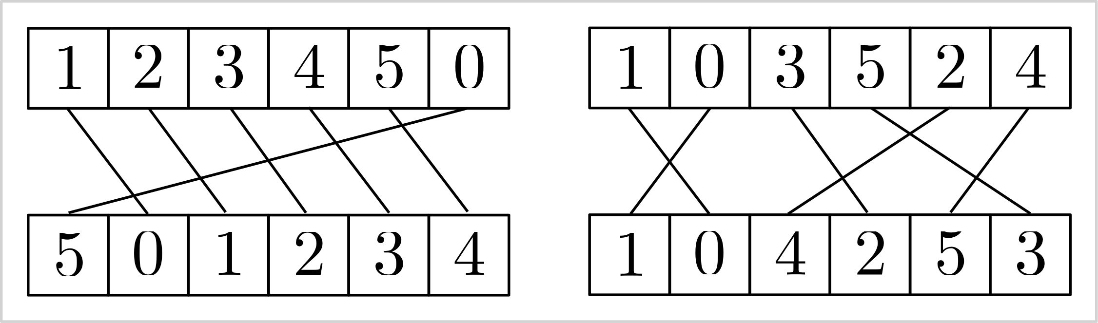 |
|---|
Visualizing the stable matching induced by the add_inverse constraint. |
[!WARNING]
I generally advise against using the
add_elementandadd_inverseconstraints. While CP-SAT may have effective propagation techniques for them, these constraints can appear unnatural and complex. It's often more straightforward to model stable matching with binary variables $x_{ij}$, indicating whether $v_i$ is matched with $w_j$, and employing anadd_exactly_oneconstraint for each vertex to ensure unique matches. If your model needs to capture specific attributes or costs associated with connections, binary variables are necessary. Relying solely on indices would require additional logic for accurate representation. Additionally, use non-binary variables only if the numerical value inherently carries semantic meaning that cannot simply be re-indexed.
Advanced Modeling
After having seen the basic elements of CP-SAT, this chapter will introduce you to the more complex constraints. These constraints are already focused on specific problems, such as routing or scheduling, but very generic and powerful within their domain. However, they also need more explanation on the correct usage.
- Tour Constraints:
add_circuit,add_multiple_circuit - Automaton Constraints:
add_automaton - Reservoir Constraints:
add_reservoir_constraint,add_reservoir_constraint_with_active - Intervals:
new_interval_var,new_interval_var_series,new_fixed_size_interval_var,new_optional_interval_var,new_optional_interval_var_series,new_optional_fixed_size_interval_var,new_optional_fixed_size_interval_var_series,add_no_overlap,add_no_overlap_2d,add_cumulative - Piecewise Linear Constraints: Not officially part of CP-SAT, but we provide some free copy&pasted code to do it.
Circuit/Tour-Constraints
Routes and tours are essential in addressing optimization challenges across
various fields, far beyond traditional routing issues. For example, in DNA
sequencing, optimizing the sequence in which DNA fragments are assembled is
crucial, while in scientific research, methodically ordering the reconfiguration
of experiments can greatly reduce operational costs and downtime. The
add_circuit and add_multiple_circuit constraints in CP-SAT allow you to
easily model various scenarios. These constraints extend beyond the classical
Traveling Salesman Problem (TSP),
allowing for solutions where not every node needs to be visited and
accommodating scenarios that require multiple disjoint sub-tours. This
adaptability makes them invaluable for a broad spectrum of practical problems
where the sequence and arrangement of operations critically impact efficiency
and outcomes.
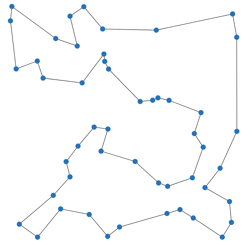 |
|---|
| The Traveling Salesman Problem (TSP) asks for the shortest possible route that visits every vertex exactly once and returns to the starting vertex. |
The Traveling Salesman Problem is one of the most famous and well-studied combinatorial optimization problems. It is a classic example of a problem that is easy to understand, common in practice, but hard to solve. It also has a special place in the history of optimization, as many techniques that are now used generally were first developed for the TSP. If you have not done so yet, I recommend watching this talk by Bill Cook, or even reading the book In Pursuit of the Traveling Salesman.
[!TIP]
If your problem is specifically the Traveling Salesperson Problem (TSP), you might find the Concorde solver particularly effective. For problems closely related to the TSP, a Mixed Integer Programming (MIP) solver may be more suitable, as many TSP variants yield strong linear programming relaxations that MIP solvers can efficiently exploit. Additionally, consider OR-Tools Routing if routing constitutes a significant aspect of your problem. However, for scenarios where variants of the TSP are merely a component of a larger problem, utilizing CP-SAT with the
add_circuitoradd_multiple_circuitconstraints can be very beneficial.
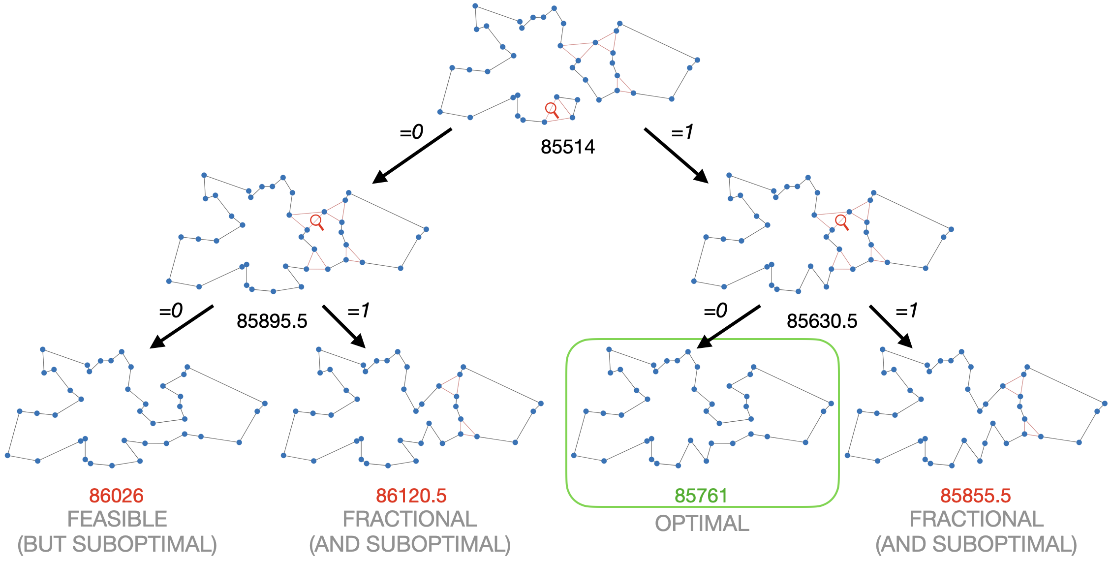 |
|---|
| This example shows why Mixed Integer Programming solvers are so good in solving the TSP. The linear relaxation (at the top) is already very close to the optimal solution. By branching, i.e., trying 0 and 1, on just two fractional variables, we not only find the optimal solution but can also prove optimality. The example was generated with the DIY TSP Solver. |
add_circuit
The add_circuit constraint is utilized to solve circuit problems within
directed graphs, even allowing loops. It operates by taking a list of triples
(u,v,var), where u and v denote the source and target vertices,
respectively, and var is a Boolean variable that indicates if an edge is
included in the solution. The constraint ensures that the edges marked as True
form a single circuit visiting each vertex exactly once, aside from vertices
with a loop set as True. Vertex indices should start at 0 and must not be
skipped to avoid isolation and infeasibility in the circuit.
Here is an example using the CP-SAT solver to address a directed Traveling Salesperson Problem (TSP):
from ortools.sat.python import cp_model

# Directed graph with weighted edges
dgraph = {(0, 1): 13, (1, 0): 17, ...(2, 3): 27}

# Initialize CP-SAT model
model = cp_model.CpModel()

# Boolean variables for each edge
edge_vars = {(u, v): model.new_bool_var(f"e_{u}_{v}") for (u, v) in dgraph.keys()}

# Circuit constraint for a single tour
model.add_circuit([(u, v, var) for (u, v), var in edge_vars.items()])

# Objective function to minimize total cost
model.minimize(sum(dgraph[(u, v)] * x for (u, v), x in edge_vars.items()))

# Solve model
solver = cp_model.CpSolver()
status = solver.solve(model)
if status in (cp_model.OPTIMAL, cp_model.FEASIBLE):
    tour = [(u, v) for (u, v), x in edge_vars.items() if solver.value(x)]
    print("Tour:", tour)

# Output: [(0, 1), (2, 0), (3, 2), (1, 3)], i.e., 0 -> 1 -> 3 -> 2 -> 0
This constraint can be adapted for paths by adding a virtual enforced edge that
closes the path into a circuit, such as (3, 0, 1) for a path from vertex 0 to
vertex 3.
Creative usage of add_circuit
The add_circuit constraint can be creatively adapted to solve various related
problems. While there are more efficient algorithms for solving the Shortest
Path Problem, let us demonstrate how to adapt the add_circuit constraint for
educational purposes.
from ortools.sat.python import cp_model

# Define a weighted, directed graph with edge costs
dgraph = {(0, 1): 13, (1, 0): 17, ...(2, 3): 27}

source_vertex = 0
target_vertex = 3

# Add zero-cost loops for vertices not being the source or target
for v in [1, 2]:
    dgraph[(v, v)] = 0

# Initialize CP-SAT model and variables
model = cp_model.CpModel()
edge_vars = {(u, v): model.new_bool_var(f"e_{u}_{v}") for (u, v) in dgraph}

# Define the circuit including a pseudo-edge from target to source
circuit = [(u, v, var) for (u, v), var in edge_vars.items()] + [
    (target_vertex, source_vertex, 1)
]
model.add_circuit(circuit)

# Minimize total cost
model.minimize(sum(dgraph[(u, v)] * x for (u, v), x in edge_vars.items()))

# Solve and extract the path
solver = cp_model.CpSolver()
status = solver.solve(model)
if status in (cp_model.OPTIMAL, cp_model.FEASIBLE):
    path = [(u, v) for (u, v), x in edge_vars.items() if solver.value(x) and u != v]
    print("Path:", path)

# Output: [(0, 1), (1, 3)], i.e., 0 -> 1 -> 3
This approach showcases the flexibility of the add_circuit constraint for
various tour and path problems. Explore further examples:
- Budget constrained tours: Optimize the largest possible tour within a specified budget.
- Multiple tours: Solve for $k$ minimal tours covering all vertices.
add_multiple_circuit
You can model multiple disjoint tours using several add_circuit constraints,
as demonstrated in
this example.
If all tours share a common depot (vertex 0), the add_multiple_circuit
constraint is an alternative. However, this constraint does not allow you to
specify the number of tours, nor can it determine to which tour a particular
edge belongs. Therefore, the add_circuit constraint is often a superior
choice. Although the arguments for both constraints are identical, vertex 0
serves a unique role as the depot where all tours commence and conclude.
Performance of add_circuit for the TSP
The table below displays the performance of the CP-SAT solver on various
instances of the TSPLIB, using the add_circuit constraint, under a 90-second
time limit. The performance can be considered reasonable, but can be easily
beaten by a Mixed Integer Programming solver.
| Instance | # vertices | runtime | lower bound | objective | opt. gap |
|---|---|---|---|---|---|
| att48 | 48 | 0.47 | 33522 | 33522 | 0 |
| eil51 | 51 | 0.69 | 426 | 426 | 0 |
| st70 | 70 | 0.8 | 675 | 675 | 0 |
| eil76 | 76 | 2.49 | 538 | 538 | 0 |
| pr76 | 76 | 54.36 | 108159 | 108159 | 0 |
| kroD100 | 100 | 9.72 | 21294 | 21294 | 0 |
| kroC100 | 100 | 5.57 | 20749 | 20749 | 0 |
| kroB100 | 100 | 6.2 | 22141 | 22141 | 0 |
| kroE100 | 100 | 9.06 | 22049 | 22068 | 0 |
| kroA100 | 100 | 8.41 | 21282 | 21282 | 0 |
| eil101 | 101 | 2.24 | 629 | 629 | 0 |
| lin105 | 105 | 1.37 | 14379 | 14379 | 0 |
| pr107 | 107 | 1.2 | 44303 | 44303 | 0 |
| pr124 | 124 | 33.8 | 59009 | 59030 | 0 |
| pr136 | 136 | 35.98 | 96767 | 96861 | 0 |
| pr144 | 144 | 21.27 | 58534 | 58571 | 0 |
| kroB150 | 150 | 58.44 | 26130 | 26130 | 0 |
| kroA150 | 150 | 90.94 | 26498 | 26977 | 2% |
| pr152 | 152 | 15.28 | 73682 | 73682 | 0 |
| kroA200 | 200 | 90.99 | 29209 | 29459 | 1% |
| kroB200 | 200 | 31.69 | 29437 | 29437 | 0 |
| pr226 | 226 | 74.61 | 80369 | 80369 | 0 |
| gil262 | 262 | 91.58 | 2365 | 2416 | 2% |
| pr264 | 264 | 92.03 | 49121 | 49512 | 1% |
| pr299 | 299 | 92.18 | 47709 | 49217 | 3% |
| linhp318 | 318 | 92.45 | 41915 | 52032 | 19% |
| lin318 | 318 | 92.43 | 41915 | 52025 | 19% |
| pr439 | 439 | 94.22 | 105610 | 163452 | 35% |
There are two prominent formulations to model the Traveling Salesman Problem
(TSP) without an add_circuit constraint: the
Dantzig-Fulkerson-Johnson (DFJ) formulation
and the
Miller-Tucker-Zemlin (MTZ) formulation.
The DFJ formulation is generally regarded as more efficient due to its stronger
linear relaxation. However, it requires lazy constraints, which are not
supported by the CP-SAT solver. When implemented without lazy constraints, the
performance of the DFJ formulation is comparable to that of the MTZ formulation
in CP-SAT. Nevertheless, both formulations perform significantly worse than the
add_circuit constraint. This indicates the superiority of using the
add_circuit constraint for handling tours and paths in such problems. Unlike
end users, the add_circuit constraint can utilize lazy constraints internally,
offering a substantial advantage in solving the TSP.
Automaton Constraints
Automaton constraints model finite state machines, enabling the representation of feasible transitions between states. This is particularly useful in software verification, where it is essential to ensure that a program follows a specified sequence of states. Given the critical importance of verification in research, there is likely a dedicated audience that appreciates this constraint. However, others may prefer to proceed to the next section.
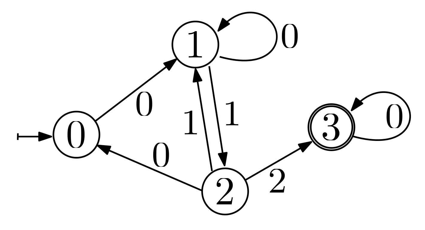 |
|---|
| An example of a finite state machine with four states and seven transitions. State 0 is the initial state, and state 3 is the final state. |
The automaton operates as follows: We have a list of integer variables
transition_variables that represent the transition values. Starting from the
starting_state, the next state is determined by the transition triple
(state, transition_value, next_state) matching the first transition variable.
If no such triple is found, the model is infeasible. This process repeats for
each subsequent transition variable. It is crucial that the final transition
leads to a final state (possibly via a loop); otherwise, the model remains
infeasible.
The state machine from the example can be modeled as follows:
model = cp_model.CpModel()

transition_variables = [model.new_int_var(0, 2, f"transition_{i}") for i in range(4)]
transition_triples = [
    (0, 0, 1),  # If in state 0 and the transition value is 0, go to state 1
    (1, 0, 1),  # If in state 1 and the transition value is 0, stay in state 1
    (1, 1, 2),  # If in state 1 and the transition value is 1, go to state 2
    (2, 0, 0),  # If in state 2 and the transition value is 0, go to state 0
    (2, 1, 1),  # If in state 2 and the transition value is 1, go to state 1
    (2, 2, 3),  # If in state 2 and the transition value is 2, go to state 3
    (3, 0, 3),  # If in state 3 and the transition value is 0, stay in state 3
]

model.add_automaton(
    transition_variables=transition_variables,
    starting_state=0,
    final_states=[3],
    transition_triples=transition_triples,
)
The assignment [0, 1, 2, 0] would be a feasible solution for this model,
whereas the assignment [1, 0, 1, 2] would be infeasible because state 0 has no
transition for value 1. Similarly, the assignment [0, 0, 1, 1] would be
infeasible as it does not end in a final state.
Reservoir Constraints
Sometimes, we need to keep the balance between inflows and outflows of a
reservoir. The name giving example is a water reservoir, where we need to keep
the water level between a minimum and a maximum level. However, there are many
other examples, such as maintaining a certain stock level in a warehouse, or
ensuring a certain staffing level in a clinic. The add_reservoir_constraint
constraint in CP-SAT allows you to model such problems easily. It takes a list
of time variables, a list of change variables, and the minimum and maximum level
of the reservoir. time_vars[i] represents the time at which the change
change_vars[i] will be applied, thus both lists needs to be of the same
length. The reservoir level starts at 0, and the minimum level has to be
$\leq 0$ and the maximum level has to be $\geq 0$.
time_vars = [model.new_int_var(0, 100, f"time_{i}") for i in range(10)]
change_vars = [model.new_int_var(-10, 10, f"change_{i}") for i in range(10)]

model.add_reservoir_constraint(
    time_vars=time_vars,
    change_vars=change_vars,
    min_level=-20,
    max_level=20,
)
Additionally, the add_reservoir_constraint_with_active constraint allows you
to model a reservoir with optional changes. Here, we additionally have a list
of Boolean variables active_vars, where active_vars[i] indicates if the
change change_vars[i] takes place. If a change is not active, it is as if it
does not exist, and the reservoir level remains the same, independent of the
time and change values.
time_vars = [model.new_int_var(0, 100, f"time_{i}") for i in range(10)]
change_vars = [model.new_int_var(-10, 10, f"change_{i}") for i in range(10)]
active_vars = [model.new_bool_var(f"active_{i}") for i in range(10)]

model.add_reservoir_constraint_with_active(
    time_vars=time_vars,
    change_vars=change_vars,
    active_vars=active_vars,
    min_level=-20,
    max_level=20,
)
[!NOTE]
The reservoir constraints can express conditions that are difficult to model "by hand". However, while I do not have much experience with them, I would not expect them to be particularly easy to optimize. Let me know if you have either good or bad experiences with them in practice and for which problem scales they work well.
Scheduling and Packing with Intervals
A special case of variables are the interval variables, that allow to model intervals, i.e., a span of some length with a start and an end. There are fixed length intervals, flexible length intervals, and optional intervals to model various use cases. These intervals become interesting in combination with the no-overlap constraints for 1D and 2D. We can use this for geometric packing problems, scheduling problems, and many other problems, where we have to prevent overlaps between intervals. These variables are special because they are actually not a variable, but a container that bounds separately defined start, length, and end variables.
There are four types of interval variables: new_interval_var,
new_fixed_size_interval_var, new_optional_interval_var, and
new_optional_fixed_size_interval_var. The new_optional_interval_var is the
most expressive but also the most expensive, while new_fixed_size_interval_var
is the least expressive and the easiest to optimize. All four types take a
start= variable. Intervals with fixed_size in their name require a constant
size= argument defining the interval length. Otherwise, the size= argument
can be a variable in combination with an end= variable, which complicates the
solution. Intervals with optional in their name include an is_present=
argument, a boolean indicating if the interval is present. The no-overlap
constraints, discussed later, apply only to intervals that are present, allowing
for modeling problems with multiple resources or optional tasks. Instead of a
pure integer variable, all arguments also accept an affine expression, e.g.,
start=5*start_var+3.
model = cp_model.CpModel()

start_var = model.new_int_var(0, 100, "start")
length_var = model.new_int_var(10, 20, "length")
end_var = model.new_int_var(0, 100, "end")
is_present_var = model.new_bool_var("is_present")

# creating an interval whose length can be influenced by a variable (more expensive)
flexible_interval = model.new_interval_var(
    start=start_var, size=length_var, end=end_var, name="flexible_interval"
)

# creating an interval of fixed length
fixed_interval = model.new_fixed_size_interval_var(
    start=start_var,
    size=10,  # needs to be a constant
    name="fixed_interval",
)

# creating an interval that can be present or not and whose length can be influenced by a variable (most expensive)
optional_interval = model.new_optional_interval_var(
    start=start_var,
    size=length_var,
    end=end_var,
    is_present=is_present_var,
    name="optional_interval",
)

# creating an interval that can be present or not
optional_fixed_interval = model.new_optional_fixed_size_interval_var(
    start=start_var,
    size=10,  # needs to be a constant
    is_present=is_present_var,
    name="optional_fixed_interval",
)
These interval variables are not useful on their own, as we could have easily achieved the same with a simple linear constraint. However, CP-SAT provides special constraints for these interval variables, that would actually be much harder to model by hand and are also much more efficient.
CP-SAT offers the following three constraints for intervals:
add_no_overlap,add_no_overlap_2d, add_cumulative. add_no_overlap is used
to prevent overlaps between intervals on a single dimension, e.g., time.
add_no_overlap_2d is used to prevent overlaps between intervals on two
dimensions, e.g., for packing rectangles. add_cumulative is used to model a
resource constraint, where the sum of the demands of the overlapping intervals
must not exceed the capacity of the resource.
The add_no_overlap constraints takes a list of (optional) interval variables
and ensures that no two present intervals overlap.
model.add_no_overlap(
    interval_vars=[
        flexible_interval,
        fixed_interval,
        optional_interval,
        optional_fixed_interval,
        # ...
    ]
)
The add_no_overlap_2d constraints takes two lists of (optional) interval and
ensures that for every i and j either x_intervals[i] and x_intervals[j]
or y_intervals[i] and y_intervals[j] do not overlap. Thus, both lists must
have the same length as x_intervals[i] and y_intervals[i] are considered
belonging together. If either x_intervals[i] or y_intervals[i] are optional,
the whole object is optional.
model.add_no_overlap_2d(
    x_intervals=[
        flexible_interval,
        fixed_interval,
        optional_interval,
        optional_fixed_interval,
        # ...
    ],
    y_intervals=[
        flexible_interval,
        fixed_interval,
        optional_interval,
        optional_fixed_interval,
        # ...
    ],
)
The add_cumulative constraint is used to model a resource constraint, where
the sum of the demands of the overlapping intervals must not exceed the capacity
of the resource. An example could be scheduling the usage of certain energy
intensive machines, where the sum of the energy demands must not exceed the
capacity of the power grid. It takes a list of intervals, a list of demands, and
a capacity variable. The list of demands must have the same length as the list
of intervals, as the demands of the intervals are matched by index. As capacity
and demands can be variables (or affine expressions), quite complex resource
constraints can be modeled.
demand_vars = [model.new_int_var(1, 10, f"demand_{i}") for i in range(4)]
capacity_var = model.new_int_var(1, 100, "capacity")
model.add_cumulative(
    intervals=[
        flexible_interval,
        fixed_interval,
        optional_interval,
        optional_fixed_interval,
    ],
    demands=demand_vars,
    capacity=capacity_var,
)
[!WARNING]
Do not directly jump to intervals when you have a scheduling problem. Intervals are great if you actually have a somewhat continuous time or space that you need to schedule. If you have a more discrete problem, such as a scheduling problem with a fixed number of slots, you can often model this problem much more efficiently using simple Boolean variables and constraints. Especially if you can use domain knowledge to find clusters of meetings that cannot overlap, this can be much more efficient.
Let us examine a few examples of how to use these constraints effectively.
Scheduling for a Conference Room with Intervals
Assume we have a conference room and need to schedule several meetings. Each
meeting has a fixed length and a range of possible start times. The time slots
are in 5-minute intervals starting at 8:00 AM and ending at 6:00 PM. Thus, there
are $10 \times 12 = 120$ time slots, and we can use a simple integer variable to
model the start time. With fixed meeting lengths, we can use the
new_fixed_size_interval_var to model the intervals. The add_no_overlap
constraint ensures no two meetings overlap, and domains for the start time can
model the range of possible start times.
To handle input data, let us define a namedtuple to store the meeting and two
functions to convert between time and index.
# Convert time to index and back
def t_to_idx(hour, minute):
    return (hour - 8) * 12 + minute // 5

def idx_to_t(time_idx):
    hour = 8 + time_idx // 12
    minute = (time_idx % 12) * 5
    return f"{hour}:{minute:02d}"

# Define meeting information using namedtuples
MeetingInfo = namedtuple("MeetingInfo", ["start_times", "duration"])
Then let us create a few meetings we want to schedule.
# Meeting definitions
meetings = {
    "meeting_a": MeetingInfo(
        start_times=[
            [t_to_idx(8, 0), t_to_idx(12, 0)],
            [t_to_idx(16, 0), t_to_idx(17, 0)],
        ],
        duration=120 // 5,  # 2 hours
    ),
    "meeting_b": MeetingInfo(
        start_times=[
            [t_to_idx(10, 0), t_to_idx(12, 0)],
        ],
        duration=30 // 5,  # 30 minutes
    ),
    "meeting_c": MeetingInfo(
        start_times=[
            [t_to_idx(16, 0), t_to_idx(17, 0)],
        ],
        duration=15 // 5,  # 15 minutes
    ),
    "meeting_d": MeetingInfo(
        start_times=[
            [t_to_idx(8, 0), t_to_idx(10, 0)],
            [t_to_idx(12, 0), t_to_idx(14, 0)],
        ],
        duration=60 // 5,  # 1 hour
    ),
}
Now we can create the CP-SAT model and add the intervals and constraints.
# Create a new CP-SAT model
model = cp_model.CpModel()

# Create start time variables for each meeting
start_time_vars = {
    meeting_name: model.new_int_var_from_domain(
        cp_model.Domain.from_intervals(meeting_info.start_times),
        f"start_{meeting_name}",
    )
    for meeting_name, meeting_info in meetings.items()
}

# Create interval variables for each meeting
interval_vars = {
    meeting_name: model.new_fixed_size_interval_var(
        start=start_time_vars[meeting_name],
        size=meeting_info.duration,
        name=f"interval_{meeting_name}",
    )
    for meeting_name, meeting_info in meetings.items()
}

# Ensure that now two meetings overlap
model.add_no_overlap(list(interval_vars.values()))
And finally, we can solve the model and extract the solution.
# Solve the model
solver = cp_model.CpSolver()
status = solver.solve(model)

# Extract and print the solution
scheduled_times = {}
if status in (cp_model.OPTIMAL, cp_model.FEASIBLE):
    for meeting_name in meetings:
        start_time = solver.value(start_time_vars[meeting_name])
        scheduled_times[meeting_name] = start_time
        print(f"{meeting_name} starts at {idx_to_t(start_time)}")
else:
    print("No feasible solution found.")
Doing some quick magic with matplotlib, we can visualize the schedule.
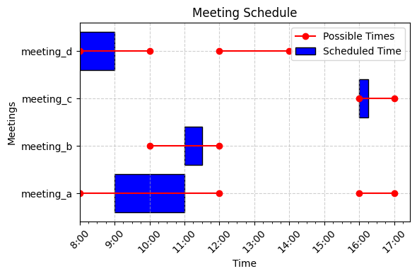 |
|---|
| A possible non-overlapping schedule for the above example. The instance is quite simple, but you could try adding some more meetings. |
Scheduling for Multiple Resources with Optional Intervals
Now, imagine we have multiple resources, such as multiple conference rooms, and
we need to schedule the meetings such that no two meetings overlap in the same
room. This can be modeled with optional intervals, where the intervals exist
only if the meeting is scheduled in the room. The add_no_overlap constraint
ensures that no two meetings overlap in the same room.
Because we now have two rooms, we need to create a more challenging instance first. Otherwise, the solver may not need to use both rooms. We do this by simply adding more and longer meetings.
# Meeting definitions
meetings = {
    "meeting_a": MeetingInfo(
        start_times=[
            [t_to_idx(8, 0), t_to_idx(12, 0)],
            [t_to_idx(16, 0), t_to_idx(16, 0)],
        ],
        duration=120 // 5,
    ),
    "meeting_b": MeetingInfo(
        start_times=[[t_to_idx(10, 0), t_to_idx(12, 0)]], duration=240 // 5
    ),
    "meeting_c": MeetingInfo(
        start_times=[[t_to_idx(16, 0), t_to_idx(17, 0)]], duration=30 // 5
    ),
    "meeting_d": MeetingInfo(
        start_times=[
            [t_to_idx(8, 0), t_to_idx(10, 0)],
            [t_to_idx(12, 0), t_to_idx(14, 0)],
        ],
        duration=60 // 5,
    ),
    "meeting_e": MeetingInfo(
        start_times=[[t_to_idx(10, 0), t_to_idx(12, 0)]], duration=120 // 5
    ),
    "meeting_f": MeetingInfo(
        start_times=[[t_to_idx(14, 0), t_to_idx(14, 0)]], duration=240 // 5
    ),
    "meeting_g": MeetingInfo(
        start_times=[[t_to_idx(14, 0), t_to_idx(16, 0)]], duration=120 // 5
    ),
}
This time, we need to create an interval variable for each room and meeting, as well as a Boolean variable indicating if the meeting is scheduled in the room. We cannot use the same interval variable for multiple rooms, as otherwise the interval would be present in both rooms.
# Create the model
model = cp_model.CpModel()

# Create start time and room variables
start_time_vars = {
    name: model.new_int_var_from_domain(
        cp_model.Domain.from_intervals(info.start_times), f"start_{name}"
    )
    for name, info in meetings.items()
}

rooms = ["room_a", "room_b"]
room_vars = {
    name: {room: model.new_bool_var(f"{name}_in_{room}") for room in rooms}
    for name in meetings
}

# Create interval variables and add no-overlap constraint
interval_vars = {
    name: {
        # We need a separate interval for each room
        room: model.new_optional_fixed_size_interval_var(
            start=start_time_vars[name],
            size=info.duration,
            is_present=room_vars[name][room],
            name=f"interval_{name}_in_{room}",
        )
        for room in rooms
    }
    for name, info in meetings.items()
}
Now we can enforce that each meeting is assigned to exactly one room and that there is no overlap between meetings in the same room.
# Ensure each meeting is assigned to exactly one room
for name, room_dict in room_vars.items():
    model.add_exactly_one(room_dict.values())

for room in rooms:
    model.add_no_overlap([interval_vars[name][room] for name in meetings])
Again, doing some quick magic with matplotlib, we get the following schedule.
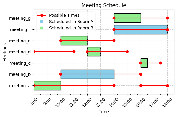 |
|---|
| A possible non-overlapping schedule for the above example with multiple rooms. |
[!TIP]
You could easily extend this model to schedule as many meetings as possible using an objective function. You could also maximize the distance between two meetings by using a variable size interval. This would be a good exercise to try.
Packing rectangles without overlaps
Let us examine how to check if a set of rectangles can be packed into a container without overlaps. This is a common problem in logistics, where boxes must be packed into a container, or in cutting stock problems, where pieces are cut from a larger material.
First, we define namedtuples for the rectangles and the container.
from collections import namedtuple

# Define namedtuples for rectangles and container
Rectangle = namedtuple("Rectangle", ["width", "height"])
Container = namedtuple("Container", ["width", "height"])

# Example usage
rectangles = [Rectangle(width=2, height=3), Rectangle(width=4, height=5)]
container = Container(width=10, height=10)
Next, we create variables for the bottom-left corners of the rectangles. These variables are constrained to ensure the rectangles remain within the container.
model = cp_model.CpModel()

# Create variables for the bottom-left corners of the rectangles
x_vars = [
    model.new_int_var(0, container.width - box.width, name=f"x1_{i}")
    for i, box in enumerate(rectangles)
]
y_vars = [
    model.new_int_var(0, container.height - box.height, name=f"y1_{i}")
    for i, box in enumerate(rectangles)
]
Next, we create interval variables for each rectangle. The start of these
intervals corresponds to the bottom-left corner, and the size is the width or
height of the rectangle. We use the add_no_overlap_2d constraint to ensure
that no two rectangles overlap.
# Create interval variables representing the width and height of the rectangles
x_interval_vars = [
    model.new_fixed_size_interval_var(
        start=x_vars[i], size=box.width, name=f"x_interval_{i}"
    )
    for i, box in enumerate(rectangles)
]
y_interval_vars = [
    model.new_fixed_size_interval_var(
        start=y_vars[i], size=box.height, name=f"y_interval_{i}"
    )
    for i, box in enumerate(rectangles)
]

# Ensure no two rectangles overlap
model.add_no_overlap_2d(x_interval_vars, y_interval_vars)
The optional intervals with flexible length allow us to model rotations and find the largest possible packing. The code may appear complex, but it remains straightforward considering the problem's complexity.
First, we define namedtuples for the rectangles and the container.
from collections import namedtuple
from ortools.sat.python import cp_model

# Define namedtuples for rectangles and container
Rectangle = namedtuple("Rectangle", ["width", "height", "value"])
Container = namedtuple("Container", ["width", "height"])

# Example usage
rectangles = [
    Rectangle(width=2, height=3, value=1),
    Rectangle(width=4, height=5, value=1),
]
container = Container(width=10, height=10)
Next, we create variables for the coordinates of the rectangles. This includes variables for the bottom-left and top-right corners, as well as a boolean variable to indicate if a rectangle is rotated.
model = cp_model.CpModel()

# Create variables for the bottom-left and top-right corners of the rectangles
bottom_left_x_vars = [
    model.new_int_var(0, container.width, name=f"x1_{i}")
    for i, box in enumerate(rectangles)
]
bottom_left_y_vars = [
    model.new_int_var(0, container.height, name=f"y1_{i}")
    for i, box in enumerate(rectangles)
]
upper_right_x_vars = [
    model.new_int_var(0, container.width, name=f"x2_{i}")
    for i, box in enumerate(rectangles)
]
upper_right_y_vars = [
    model.new_int_var(0, container.height, name=f"y2_{i}")
    for i, box in enumerate(rectangles)
]

# Create variables to indicate if a rectangle is rotated
rotated_vars = [model.new_bool_var(f"rotated_{i}") for i in range(len(rectangles))]
We then create variables for the width and height of each rectangle, adjusting for rotation. Constraints ensure these variables are set correctly based on whether the rectangle is rotated.
# Create variables for the width and height, adjusted for rotation
width_vars = []
height_vars = []
for i, box in enumerate(rectangles):
    domain = cp_model.Domain.from_values([box.width, box.height])
    width_vars.append(model.new_int_var_from_domain(domain, name=f"width_{i}"))
    height_vars.append(model.new_int_var_from_domain(domain, name=f"height_{i}"))
    # There are two possible assignments for width and height
    model.add_allowed_assignments(
        [width_vars[i], height_vars[i], rotated_vars[i]],
        [(box.width, box.height, 0), (box.height, box.width, 1)],
    )
Next, we create a boolean variable indicating if a rectangle is packed or not, and then interval variables representing its occupied space in the container. These intervals are used to enforce the no-overlap constraint.
# Create variables indicating if a rectangle is packed
packed_vars = [model.new_bool_var(f"packed_{i}") for i in range(len(rectangles))]

# Create interval variables representing the width and height of the rectangles
x_interval_vars = [
    model.new_optional_interval_var(
        start=bottom_left_x_vars[i],
        size=width_vars[i],
        is_present=packed_vars[i],
        end=upper_right_x_vars[i],
        name=f"x_interval_{i}",
    )
    for i, box in enumerate(rectangles)
]
y_interval_vars = [
    model.new_optional_interval_var(
        start=bottom_left_y_vars[i],
        size=height_vars[i],
        is_present=packed_vars[i],
        end=upper_right_y_vars[i],
        name=f"y_interval_{i}",
    )
    for i, box in enumerate(rectangles)
]

# Ensure no two rectangles overlap
model.add_no_overlap_2d(x_interval_vars, y_interval_vars)
Finally, we maximize the number of packed rectangles by defining an objective function.
# Maximize the number of packed rectangles
model.maximize(sum(box.value * x for x, box in zip(packed_vars, rectangles))) |
|---|
| This dense packing was found by CP-SAT in less than 0.3s, which is quite impressive and seems to be more efficient than a naive Gurobi implementation. |
You can find the full code here:
| Problem Variant | Code |
|---|---|
| Deciding feasibility of packing rectangles without rotations | ./evaluations/packing/solver/packing_wo_rotations.py |
| Finding the largest possible packing of rectangles without rotations | ./evaluations/packing/solver/knapsack_wo_rotations.py |
| Deciding feasibility of packing rectangles with rotations | ./evaluations/packing/solver/packing_with_rotations.py |
| Finding the largest possible packing of rectangles with rotations | ./evaluations/packing/solver/knapsack_with_rotations.py |
CP-SAT is good at finding a feasible packing, but incapable of proofing infeasibility in most cases. When using the knapsack variant, it can still pack most of the rectangles even for the larger instances.
 |
|---|
| The number of solved instances for the packing problem (90s time limit). Rotations make things slightly more difficult. None of the used instances were proofed infeasible. |
 |
| However, CP-SAT is able to pack nearly all rectangles even for the largest instances. |
Resolution and Parameters
In earlier versions of CP-SAT, the performance of no-overlap constraints was greatly influenced by the resolution. This impact has evolved, yet it remains somewhat inconsistent. In a notebook example, I explored how resolution affects the execution time of the no-overlap constraint in versions 9.3 and 9.8 of CP-SAT. For version 9.3, there is a noticeable increase in execution time as the resolution grows. Conversely, in version 9.8, execution time actually reduces when the resolution is higher, a finding supported by repeated tests. This unexpected behavior suggests that the performance of CP-SAT regarding no-overlap constraints has not stabilized and may continue to vary in upcoming versions.
| Resolution | Runtime (CP-SAT 9.3) | Runtime (CP-SAT 9.8) |
|---|---|---|
| 1x | 0.02s | 0.03s |
| 10x | 0.7s | 0.02s |
| 100x | 7.6s | 1.1s |
| 1000x | 75s | 40.3s |
| 10_000x | >15min | 0.4s |
This notebook was used to create the table above.
However, while playing around with less documented features, I noticed that the performance for the older version can be improved drastically with the following parameters:
solver.parameters.use_energetic_reasoning_in_no_overlap_2d = True
solver.parameters.use_timetabling_in_no_overlap_2d = True
solver.parameters.use_pairwise_reasoning_in_no_overlap_2d = True
With the latest version of CP-SAT, I did not notice a significant difference in performance when using these parameters.
Non-Linear Constraints/Piecewise Linear Functions
In practice, you often have cost functions that are not linear. For example, consider a production problem where you have three different items you produce. Each item has different components, you have to buy. The cost of the components will first decrease with the amount you buy, then at some point increase again as your supplier will be out of stock and you have to buy from a more expensive supplier. Additionally, you only have a certain amount of customers willing to pay a certain price for your product. If you want to sell more, you will have to lower the price, which will decrease your profit.
Let us assume such a function looks like $y=f(x)$ in the following figure. Unfortunately, it is a rather complex function that we cannot directly express in CP-SAT. However, we can approximate it with a piecewise linear function as shown in red. Such piecewise linear approximations are very common, and some solvers can even do them automatically, e.g., Gurobi. The resolution can be arbitrarily high, but the more segments you have, the more complex the model becomes. Thus, it is usually only chosen to be as high as necessary.
 |
|---|
| We can model an arbitrary continuous function with a piecewise linear function. Here, we split the original function into a number of straight segments. The accuracy can be adapted to the requirements. The linear segments can then be expressed in CP-SAT. The fewer such segments, the easier it remains to model and solve. |
Using linear constraints (model.add) and reification (.only_enforce_if), we
can model such a piecewise linear function in CP-SAT. For this we simply use
boolean variables to decide for a segment, and then activate the corresponding
linear constraint via reification. However, this has two problems in CP-SAT, as
shown in the next figure.
 |
|---|
| Even if the function f(x) now consists of linear segments, we cannot simply implement $y=f(x)$ in CP-SAT. First, for many $x$-values, $f(x)$ will be not integral and, thus, infeasible. Second, the canonical representation of many linear segments will require non-integral coefficients, which are also not allowed in CP-SAT. |
-
Problem A: Even if we can express a segment as a linear function, the result of the function may not be integral. In the example, $f(5)$ would be $3.5$ and, thus, if we enforce $y=f(x)$, $x$ would be prohibited to be $5$, which is not what we want. There are two options now. Either, we use a more complex piecewise linear approximation that ensures that the function will always yield integral solutions or we use inequalities instead. The first solution has the issue that this can require too many segments, making it far too expensive to optimize. The second solution will be a weaker constraint as now we can only enforce $y<=f(x)$ or $y>=f(x)$, but not $y=f(x)$. If you try to enforce it by $y<=f(x)$ and $y>=f(x)$, you will end with the same infeasibility as before. However, often an inequality will be enough. If the problem is to prevent $y$ from becoming too large, you use $y<=f(x)$, if the problem is to prevent $y$ from becoming too small, you use $y>=f(x)$. If we want to represent the costs by $f(x)$, we would use $y>=f(x)$ to minimize the costs.
-
Problem B: The canonical representation of a linear function is $y=ax+b$. However, this will often require non-integral coefficients. Luckily, we can automatically scale them up to integral values by adding a scaling factor. The inequality $y=0.5x+0.5$ in the example can also be represented as $2y=x+1$. I will spare you the math, but it just requires a simple trick with the least common multiple. Of course, the required scaling factor can become large, and at some point lead to overflows.
An implementation could now look as follows:
# We want to enforce y=f(x)
x = model.new_int_var(0, 7, "x")
y = model.new_int_var(0, 5, "y")

# use boolean variables to decide for a segment
segment_active = [model.new_bool_var("segment_1"), model.new_bool_var("segment_2")]
model.add_at_most_one(segment_active)  # enforce one segment to be active

# Segment 1
# if 0<=x<=3, then y >= 0.5*x + 0.5
model.add(2 * y >= x + 1).only_enforce_if(segment_active[0])
model.add(x >= 0).only_enforce_if(segment_active[0])
model.add(x <= 3).only_enforce_if(segment_active[0])

# Segment 2
model.add(_SLIGHTLY_MORE_COMPLEX_INEQUALITY_).only_enforce_if(segment_active[1])
model.add(x >= 3).only_enforce_if(segment_active[1])
model.add(x <= 7).only_enforce_if(segment_active[1])

model.minimize(y)
# if we were to maximize y, we would have used <= instead of >=
This can be quite tedious, but luckily, I wrote a small helper class that will do this automatically for you. You can find it in ./utils/piecewise_functions. Simply copy it into your code.
This code does some further optimizations:
- Considering every segment as a separate case can be quite expensive and inefficient. Thus, it can make a serious difference if you can combine multiple segments into a single case. This can be achieved by detecting convex ranges, as the constraints of convex areas do not interfere with each other.
- Adding the convex hull of the segments as a redundant constraint that does
not depend on any
only_enforce_ifcan in some cases help the solver to find better bounds.only_enforce_if-constraints are often not very good for the linear relaxation, and having the convex hull as independent constraint can directly limit the solution space, without having to do any branching on the cases.
Let us use this code to solve an instance of the problem above.
We have two products that each require three components. The first product requires 3 of component 1, 5 of component 2, and 2 of component 3. The second product requires 2 of component 1, 1 of component 2, and 3 of component 3. We can buy up to 1500 of each component for the price given in the figure below. We can produce up to 300 of each product and sell them for the price given in the figure below.
 |
 |
|---|---|
| Costs for buying components necessary for production. | Selling price for the products. |
We want to maximize the profit, i.e., the selling price minus the costs for buying the components. We can model this as follows:
requirements_1 = (3, 5, 2)
requirements_2 = (2, 1, 3)

from ortools.sat.python import cp_model

model = cp_model.CpModel()
buy_1 = model.new_int_var(0, 1_500, "buy_1")
buy_2 = model.new_int_var(0, 1_500, "buy_2")
buy_3 = model.new_int_var(0, 1_500, "buy_3")

produce_1 = model.new_int_var(0, 300, "produce_1")
produce_2 = model.new_int_var(0, 300, "produce_2")

model.add(produce_1 * requirements_1[0] + produce_2 * requirements_2[0] <= buy_1)
model.add(produce_1 * requirements_1[1] + produce_2 * requirements_2[1] <= buy_2)
model.add(produce_1 * requirements_1[2] + produce_2 * requirements_2[2] <= buy_3)

# You can find this code it ./utils!
from piecewise_functions import PiecewiseLinearFunction, PiecewiseLinearConstraint

# Define the functions for the costs
costs_1 = [(0, 0), (1000, 400), (1500, 1300)]
costs_2 = [(0, 0), (300, 300), (700, 500), (1200, 600), (1500, 1100)]
costs_3 = [(0, 0), (200, 400), (500, 700), (1000, 900), (1500, 1500)]
# PiecewiseLinearFunction is a pydantic model and can be serialized easily!
f_costs_1 = PiecewiseLinearFunction(
    xs=[x for x, y in costs_1], ys=[y for x, y in costs_1]
)
f_costs_2 = PiecewiseLinearFunction(
    xs=[x for x, y in costs_2], ys=[y for x, y in costs_2]
)
f_costs_3 = PiecewiseLinearFunction(
    xs=[x for x, y in costs_3], ys=[y for x, y in costs_3]
)

# Define the functions for the gain
gain_1 = [(0, 0), (100, 800), (200, 1600), (300, 2_000)]
gain_2 = [(0, 0), (80, 1_000), (150, 1_300), (200, 1_400), (300, 1_500)]
f_gain_1 = PiecewiseLinearFunction(xs=[x for x, y in gain_1], ys=[y for x, y in gain_1])
f_gain_2 = PiecewiseLinearFunction(xs=[x for x, y in gain_2], ys=[y for x, y in gain_2])

# Create y>=f(x) constraints for the costs
x_costs_1 = PiecewiseLinearConstraint(model, buy_1, f_costs_1, upper_bound=False)
x_costs_2 = PiecewiseLinearConstraint(model, buy_2, f_costs_2, upper_bound=False)
x_costs_3 = PiecewiseLinearConstraint(model, buy_3, f_costs_3, upper_bound=False)

# Create y<=f(x) constraints for the gain
x_gain_1 = PiecewiseLinearConstraint(model, produce_1, f_gain_1, upper_bound=True)
x_gain_2 = PiecewiseLinearConstraint(model, produce_2, f_gain_2, upper_bound=True)

# Maximize the gain minus the costs
model.Maximize(x_gain_1.y + x_gain_2.y - (x_costs_1.y + x_costs_2.y + x_costs_3.y))

solver = cp_model.CpSolver()
solver.parameters.log_search_progress = True
status = solver.solve(model)
print(f"Buy {solver.value(buy_1)} of component 1")
print(f"Buy {solver.value(buy_2)} of component 2")
print(f"Buy {solver.value(buy_3)} of component 3")
print(f"Produce {solver.value(produce_1)} of product 1")
print(f"Produce {solver.value(produce_2)} of product 2")
print(f"Overall gain: {solver.objective_value}")
This will give you the following output:
Buy 930 of component 1
Buy 1200 of component 2
Buy 870 of component 3
Produce 210 of product 1
Produce 150 of product 2
Overall gain: 1120.0
Unfortunately, these problems quickly get very complicated to model and solve. This is just a proof that, theoretically, you can model such problems in CP-SAT. Practically, you can lose a lot of time and sanity with this if you are not an expert.
Parameters
The CP-SAT solver offers numerous parameters to control its behavior. These
parameters are implemented via
Protocol Buffers and can be
manipulated using the parameters member. To explore all available options,
refer to the well-documented proto file in the
official repository.
Below, I will highlight the most important parameters so you can get the most
out of CP-SAT.
:warning: Only a few parameters, such as
max_time_in_seconds, are suitable for beginners. Most other parameters, like decision strategies, are best left at their default settings, as they are well-chosen and tampering with them could disrupt optimizations. For better performance, focus on improving your model.
Logging
The log_search_progress parameter is crucial at the beginning. It enables
logging of the search progress, providing insights into how CP-SAT solves your
problem. While you may deactivate it later for production, it is beneficial
during development to understand the process and respond to any issues.
solver = cp_model.CpSolver()
solver.parameters.log_search_progress = True

# Custom log function, for example, using the Python logging module instead of stdout
# Useful in a Jupyter notebook, where logging to stdout might not be visible
solver.log_callback = print  # (str)->None
# If using a custom log function, you can disable logging to stdout
solver.parameters.log_to_stdout = False
The log offers valuable information for understanding CP-SAT and your optimization problem. It details aspects such as how many variables were directly removed and which techniques most effectively contributed to improving lower and upper bounds.
An example log might look like this:
Starting CP-SAT solver v9.10.4067
Parameters: max_time_in_seconds: 30 log_search_progress: true relative_gap_limit: 0.01
Setting number of workers to 16

Initial optimization model '': (model_fingerprint: 0x1d316fc2ae4c02b1)
#Variables: 450 (#bools: 276 #ints: 6 in objective)
  - 342 Booleans in [0,1]
  - 12 in [0][10][20][30][40][50][60][70][80][90][100]
  - 6 in [0][10][20][30][40][100]
  - 6 in [0][80][100]
  - 6 in [0][100]
  - 6 in [0,1][34][67][100]
  - 12 in [0,6]
  - 18 in [0,7]
  - 6 in [0,35]
  - 6 in [0,36]
  - 6 in [0,100]
  - 12 in [21,57]
  - 12 in [22,57]
#kBoolOr: 30 (#literals: 72)
#kLinear1: 33 (#enforced: 12)
#kLinear2: 1'811
#kLinear3: 36
#kLinearN: 94 (#terms: 1'392)

Starting presolve at 0.00s
  3.26e-04s  0.00e+00d  [DetectDominanceRelations]
  6.60e-03s  0.00e+00d  [PresolveToFixPoint] #num_loops=4 #num_dual_strengthening=3
  2.69e-05s  0.00e+00d  [ExtractEncodingFromLinear] #potential_supersets=44 #potential_subsets=12
[Symmetry] Graph for symmetry has 2'224 nodes and 5'046 arcs.
[Symmetry] Symmetry computation done. time: 0.000374304 dtime: 0.00068988
[Symmetry] #generators: 2, average support size: 12
[Symmetry] 12 orbits with sizes: 2,2,2,2,2,2,2,2,2,2,...
[Symmetry] Found orbitope of size 6 x 2
[SAT presolve] num removable Booleans: 0 / 309
[SAT presolve] num trivial clauses: 0
[SAT presolve] [0s] clauses:570 literals:1152 vars:303 one_side_vars:268 simple_definition:35 singleton_clauses:0
[SAT presolve] [3.0778e-05s] clauses:570 literals:1152 vars:303 one_side_vars:268 simple_definition:35 singleton_clauses:0
[SAT presolve] [4.6758e-05s] clauses:570 literals:1152 vars:303 one_side_vars:268 simple_definition:35 singleton_clauses:0
  1.10e-02s  9.68e-03d  [Probe] #probed=1'738 #new_bounds=12 #new_binary_clauses=1'111
  2.34e-03s  0.00e+00d  [MaxClique] Merged 602(1374 literals) into 506(1960 literals) at_most_ones.
  3.31e-04s  0.00e+00d  [DetectDominanceRelations]
  1.89e-03s  0.00e+00d  [PresolveToFixPoint] #num_loops=2 #num_dual_strengthening=1
  5.45e-04s  0.00e+00d  [ProcessAtMostOneAndLinear]
  8.19e-04s  0.00e+00d  [DetectDuplicateConstraints] #without_enforcements=306
  8.62e-05s  7.21e-06d  [DetectDominatedLinearConstraints] #relevant_constraints=114 #num_inclusions=42
  1.94e-05s  0.00e+00d  [DetectDifferentVariables]
  1.90e-04s  8.39e-06d  [ProcessSetPPC] #relevant_constraints=560 #num_inclusions=24
  2.01e-05s  0.00e+00d  [FindAlmostIdenticalLinearConstraints]
...
Given the complexity of the log, I developed a tool to visualize and comment on it. You can copy and paste your log into the tool, which will automatically highlight the most important details. Be sure to check out the examples.
![]()
 |
|---|
| A plot of the search progress over time as visualized by the log analyzer using information from the log (a different log than displayed above). This plot helps you understand which part of your problem is more challenging: finding a good solution or proving its quality. Based on this, you can implement appropriate countermeasures. |
We will revisit the logs in the next chapter.
[!TIP]
From my experience as a lecturer, I often encounter students who believe CP-SAT is stuck, only to discover that their model building includes an unnecessarily complex $O(n^5)$ nested loop, which would take days to run. It is natural to assume that the issue lies with CP-SAT because it handles the hard part of solving the problem. However, even the seemingly simple part of model building can consume a lot of time if implemented incorrectly. By enabling logging, students could immediately see that the issue lies in their own code rather than with CP-SAT. This simple step can save a lot of time and frustration.
Time Limit and Status
When working with large or complex models, the CP-SAT solver may not always reach an optimal solution within a reasonable time frame and could potentially run indefinitely. Therefore, setting a time limit is advisable, particularly in a production environment, to prevent the solver from running endlessly. Even within a time limit, CP-SAT often finds a reasonably good solution, although it may not be proven optimal.
Determining an appropriate time limit depends on various factors and usually requires some experimentation. I typically start with a time limit between 60 and 300 seconds, as this provides a balance between not having to wait too long during model testing and giving the solver enough time to find a good solution.
To set a time limit (in seconds) before running the solver, use the following command:
# solver = cp_model.CpSolver()
solver.parameters.max_time_in_seconds = 60  # 60s time limit
# status = solver.solve(model)
After running the solver, it is important to check the status to determine whether an optimal solution, a feasible solution, or no solution at all has been found:
status = solver.solve(model)
if status == cp_model.OPTIMAL or status == cp_model.FEASIBLE:
    print("We have a solution.")
else:
    print("Help?! No solution available! :( ")
The possible status codes are:
OPTIMAL(4): An optimal solution has been found.FEASIBLE(2): A feasible solution has been found, and a bound may be available to assess its quality viasolver.best_objective_bound.INFEASIBLE(3): No solution can satisfy all constraints.MODEL_INVALID(1): The CP-SAT model is incorrectly specified.UNKNOWN(0): No solution was found, and no infeasibility proof is available. A bound may still be available.
To get the name from the status code, use solver.status_name(status).
In addition to limiting runtime, you can specify acceptable solution quality
using absolute_gap_limit and relative_gap_limit. The absolute limit stops
the solver when the solution is within a specified value of the bound. The
relative limit stops the solver when the objective value (O) is within a
specified ratio of the bound (B). To stop when the solution is (provably) within
5% of the optimum, use:
solver.parameters.relative_gap_limit = 0.05For cases where progress stalls or for other reasons, solution callbacks can be used to halt the solver. With these, you can decide on every new solution if the solution is good enough or if the solver should continue searching for a better one. Unlike Gurobi, CP-SAT does not support adding lazy constraints from these callbacks (or at all), which is a significant limitation for problems requiring dynamic model adjustments.
To add a solution callback, inherit from the base class
CpSolverSolutionCallback. Documentation for this base class and its operations
is available
here.
class MySolutionCallback(cp_model.CpSolverSolutionCallback):
    def __init__(self, data):
        cp_model.CpSolverSolutionCallback.__init__(self)
        self.data = data  # Store data in the callback.

    def on_solution_callback(self):
        obj = self.objective_value  # Best solution value
        bound = self.best_objective_bound  # Best bound
        print(f"The current value of x is {self.Value(x)}")
        if abs(obj - bound) < 10:
            self.StopSearch()  # Stop search for a better solution
        # ...

solver.solve(model, MySolutionCallback(None))
An official example using callbacks is available.
Besides querying the objective value of the best solution and the best known
bound, you can also access internal metrics such as self.num_booleans,
self.num_branches, and self.num_conflicts. These metrics will be discussed
later.
As of version 9.10, CP-SAT also supports bound callbacks, which are triggered when the proven bound improves. Unlike solution callbacks, which activate upon finding new solutions, bound callbacks are useful for stopping the search when the bound is sufficiently good. The syntax for bound callbacks differs from that of solution callbacks, as they are implemented as free functions that directly access the solver object.
solver = cp_model.CpSolver()

def bound_callback(bound):
    print(f"New bound: {bound}")
    if bound > 100:
        solver.stop_search()

solver.best_bound_callback = bound_callback
Instead of using a simple function, you can also use a callable object to store a reference to the solver object. This approach allows you to define the callback outside the local scope, providing greater flexibility.
class BoundCallback:
    def __init__(self, solver) -> None:
        self.solver = solver

    def __call__(self, bound):
        print(f"New bound: {bound}")
        if bound > 200:
            print("Abort search due to bound")
            self.solver.stop_search()
This method is more flexible than the solution callback and can be considered more Pythonic.
Additionally, whenever there is a new solution or bound, a log message is generated. You can hook into the log output to decide when to stop the search using CP-SAT's log callback.
solver.parameters.log_search_progress = True  # Enable logging
solver.log_callback = lambda msg: print("LOG:", msg)  # (str) -> None
Parallelization
CP-SAT is a portfolio-solver that uses different techniques to solve the problem. There is some information exchange between the different workers, but it does not split the solution space into different parts, thus, it does not parallelize the branch-and-bound algorithm as MIP-solvers do. This can lead to some redundancy in the search, but running different techniques in parallel will also increase the chance of running the right technique. Predicting which technique will be the best for a specific problem is often hard, thus, this parallelization can be quite useful.
You can control the parallelization of CP-SAT by setting the number of search workers.
solver.parameters.num_workers = 8 # use 8 coresHere are the solvers used by CP-SAT 9.9 on different parallelization levels for an optimization problem and no additional specifications (e.g., decision strategies). Note that some parameters/constraints/objectives can change the parallelization strategy. Also check the official documentation.
solver.parameters.num_workers = 1: Single-threaded search with[default_lp].- 1 full problem subsolver: [default_lp]
solver.parameters.num_workers = 2: Additional use of heuristics to support thedefault_lpsearch.- 1 full problem subsolver: [default_lp]
- 13 incomplete subsolvers: [feasibility_pump, graph_arc_lns, graph_cst_lns, graph_dec_lns, graph_var_lns, packing_precedences_lns, packing_rectangles_lns, packing_slice_lns, rins/rens, rnd_cst_lns, rnd_var_lns, scheduling_precedences_lns, violation_ls]
- 3 helper subsolvers: [neighborhood_helper, synchronization_agent, update_gap_integral]
solver.parameters.num_workers = 3: Using a second full problem solver that does not try to linearize the model.- 2 full problem subsolvers: [default_lp, no_lp]
- 13 incomplete subsolvers: [feasibility_pump, graph_arc_lns, graph_cst_lns, graph_dec_lns, graph_var_lns, packing_precedences_lns, packing_rectangles_lns, packing_slice_lns, rins/rens, rnd_cst_lns, rnd_var_lns, scheduling_precedences_lns, violation_ls]
- 3 helper subsolvers: [neighborhood_helper, synchronization_agent, update_gap_integral]
solver.parameters.num_workers = 4: Additionally using a third full problem solver that tries to linearize the model as much as possible.- 3 full problem subsolvers: [default_lp, max_lp, no_lp]
- 13 incomplete subsolvers: [feasibility_pump, graph_arc_lns, graph_cst_lns, graph_dec_lns, graph_var_lns, packing_precedences_lns, packing_rectangles_lns, packing_slice_lns, rins/rens, rnd_cst_lns, rnd_var_lns, scheduling_precedences_lns, violation_ls]
- 3 helper subsolvers: [neighborhood_helper, synchronization_agent, update_gap_integral]
solver.parameters.num_workers = 5: Additionally using a first solution subsolver.- 3 full problem subsolvers: [default_lp, max_lp, no_lp]
- 1 first solution subsolver: [fj_short_default]
- 13 incomplete subsolvers: [feasibility_pump, graph_arc_lns, graph_cst_lns, graph_dec_lns, graph_var_lns, packing_precedences_lns, packing_rectangles_lns, packing_slice_lns, rins/rens, rnd_cst_lns, rnd_var_lns, scheduling_precedences_lns, violation_ls]
- 3 helper subsolvers: [neighborhood_helper, synchronization_agent, update_gap_integral]
solver.parameters.num_workers = 6: Using a fourth full problem solverquick_restartthat does more "probing".- 4 full problem subsolvers: [default_lp, max_lp, no_lp, quick_restart]
- 1 first solution subsolver: [fj_short_default]
- 13 incomplete subsolvers: [feasibility_pump, graph_arc_lns, graph_cst_lns, graph_dec_lns, graph_var_lns, packing_precedences_lns, packing_rectangles_lns, packing_slice_lns, rins/rens, rnd_cst_lns, rnd_var_lns, scheduling_precedences_lns, violation_ls]
- 3 helper subsolvers: [neighborhood_helper, synchronization_agent, update_gap_integral]
solver.parameters.num_workers = 7:- 5 full problem subsolvers: [default_lp, max_lp, no_lp, quick_restart, reduced_costs]
- 1 first solution subsolver: [fj_short_default]
- 13 incomplete subsolvers: [feasibility_pump, graph_arc_lns, graph_cst_lns, graph_dec_lns, graph_var_lns, packing_precedences_lns, packing_rectangles_lns, packing_slice_lns, rins/rens, rnd_cst_lns, rnd_var_lns, scheduling_precedences_lns, violation_ls]
- 3 helper subsolvers: [neighborhood_helper, synchronization_agent, update_gap_integral]
solver.parameters.num_workers = 8:- 6 full problem subsolvers: [default_lp, max_lp, no_lp, quick_restart, quick_restart_no_lp, reduced_costs]
- 1 first solution subsolver: [fj_short_default]
- 13 incomplete subsolvers: [feasibility_pump, graph_arc_lns, graph_cst_lns, graph_dec_lns, graph_var_lns, packing_precedences_lns, packing_rectangles_lns, packing_slice_lns, rins/rens, rnd_cst_lns, rnd_var_lns, scheduling_precedences_lns, violation_ls]
- 3 helper subsolvers: [neighborhood_helper, synchronization_agent, update_gap_integral]
solver.parameters.num_workers = 12:- 8 full problem subsolvers: [default_lp, lb_tree_search, max_lp, no_lp, pseudo_costs, quick_restart, quick_restart_no_lp, reduced_costs]
- 3 first solution subsolvers: [fj_long_default, fj_short_default, fs_random]
- 13 incomplete subsolvers: [feasibility_pump, graph_arc_lns, graph_cst_lns, graph_dec_lns, graph_var_lns, packing_precedences_lns, packing_rectangles_lns, packing_slice_lns, rins/rens, rnd_cst_lns, rnd_var_lns, scheduling_precedences_lns, violation_ls]
- 3 helper subsolvers: [neighborhood_helper, synchronization_agent, update_gap_integral]
solver.parameters.num_workers = 16:- 11 full problem subsolvers: [default_lp, lb_tree_search, max_lp, no_lp, objective_lb_search, objective_shaving_search_no_lp, probing, pseudo_costs, quick_restart, quick_restart_no_lp, reduced_costs]
- 4 first solution subsolvers: [fj_long_default, fj_short_default, fs_random, fs_random_quick_restart]
- 13 incomplete subsolvers: [feasibility_pump, graph_arc_lns, graph_cst_lns, graph_dec_lns, graph_var_lns, packing_precedences_lns, packing_rectangles_lns, packing_slice_lns, rins/rens, rnd_cst_lns, rnd_var_lns, scheduling_precedences_lns, violation_ls]
- 3 helper subsolvers: [neighborhood_helper, synchronization_agent, update_gap_integral]
solver.parameters.num_workers = 20:- 13 full problem subsolvers: [default_lp, lb_tree_search, max_lp, no_lp, objective_lb_search, objective_shaving_search_max_lp, objective_shaving_search_no_lp, probing, probing_max_lp, pseudo_costs, quick_restart, quick_restart_no_lp, reduced_costs]
- 5 first solution subsolvers: [fj_long_default, fj_short_default, fj_short_lin_default, fs_random, fs_random_quick_restart]
- 13 incomplete subsolvers: [feasibility_pump, graph_arc_lns, graph_cst_lns, graph_dec_lns, graph_var_lns, packing_precedences_lns, packing_rectangles_lns, packing_slice_lns, rins/rens, rnd_cst_lns, rnd_var_lns, scheduling_precedences_lns, violation_ls]
- 3 helper subsolvers: [neighborhood_helper, synchronization_agent, update_gap_integral]
solver.parameters.num_workers = 32:- 15 full problem subsolvers: [default_lp, lb_tree_search, max_lp, no_lp, objective_lb_search, objective_lb_search_max_lp, objective_lb_search_no_lp, objective_shaving_search_max_lp, objective_shaving_search_no_lp, probing, probing_max_lp, pseudo_costs, quick_restart, quick_restart_no_lp, reduced_costs]
- 15 first solution subsolvers: [fj_long_default, fj_long_lin_default, fj_long_lin_random, fj_long_random, fj_short_default, fj_short_lin_default, fj_short_lin_random, fj_short_random, fs_random(2), fs_random_no_lp(2), fs_random_quick_restart(2), fs_random_quick_restart_no_lp]
- 15 incomplete subsolvers: [feasibility_pump, graph_arc_lns, graph_cst_lns, graph_dec_lns, graph_var_lns, packing_precedences_lns, packing_rectangles_lns, packing_slice_lns, rins/rens, rnd_cst_lns, rnd_var_lns, scheduling_precedences_lns, violation_ls(3)]
- 3 helper subsolvers: [neighborhood_helper, synchronization_agent, update_gap_integral]
solver.parameters.num_workers = 64:- 15 full problem subsolvers: [default_lp, lb_tree_search, max_lp, no_lp, objective_lb_search, objective_lb_search_max_lp, objective_lb_search_no_lp, objective_shaving_search_max_lp, objective_shaving_search_no_lp, probing, probing_max_lp, pseudo_costs, quick_restart, quick_restart_no_lp, reduced_costs]
- 47 first solution subsolvers: [fj_long_default(2), fj_long_lin_default(2), fj_long_lin_perturb(2), fj_long_lin_random(2), fj_long_perturb(2), fj_long_random(2), fj_short_default(2), fj_short_lin_default(2), fj_short_lin_perturb(2), fj_short_lin_random(2), fj_short_perturb(2), fj_short_random(2), fs_random(6), fs_random_no_lp(6), fs_random_quick_restart(6), fs_random_quick_restart_no_lp(5)]
- 19 incomplete subsolvers: [feasibility_pump, graph_arc_lns, graph_cst_lns, graph_dec_lns, graph_var_lns, packing_precedences_lns, packing_rectangles_lns, packing_slice_lns, rins/rens, rnd_cst_lns, rnd_var_lns, scheduling_precedences_lns, violation_ls(7)]
- 3 helper subsolvers: [neighborhood_helper, synchronization_agent, update_gap_integral]
Important steps:
- With a single worker, only the default subsolver is used.
- With two workers or more, CP-SAT starts using incomplete subsolvers, i.e., heuristics such as LNS.
- With five workers, CP-SAT will also have a first solution subsolver.
- With 23 workers, all 15 full problem subsolvers are used.
- For more than 32 workers, primarily the number of first solution subsolvers is increased.
Full problem subsolvers are solvers that search the full problem space, e.g., by a branch-and-bound algorithm. Available full problem subsolvers are:
default_lp: LCG-based search with default linearization of the model.max_lp: Same asdefault_lpbut with maximal linearization.no_lp: Same asdefault_lpbut without linearization.
lb_tree_search: This solver is focussed on improving the proven bound, not on finding better solutions. By disproving the feasibility of the cheapest nodes in the search tree, it incrementally improves the bound, but has only little chances to find better solutions.objective_lb_search: Also focussed on improving the bound by disproving the feasibility of the current lower bound.objective_lb_search_max_lp: With maximal linearization.objective_lb_search_no_lp: Without linearization.objective_shaving_search_max_lp: Should be quite similar toobjective_lb_search_max_lp.objective_shaving_search_no_lp: Should be quite similar toobjective_lb_search_no_lp.
probing: Fixing variables and seeing what happens.probing_max_lp: Same as probing but with maximal linearization.
pseudo_costs: Uses pseudo costs for branching, which are computed from historical changes in objective bounds following certain branching decisions.quick_restart: Restarts the search more eagerly. Restarts rebuild the search tree from scratch, but keep learned clauses. This allows to recover from bad decisions, and lead to smaller search trees by learning from the mistakes of the past.quick_restart_no_lp: Same asquick_restartbut without linearization.
reduced_costs: Uses the reduced costs of the linear relaxation for branching.core: A strategy from the SAT-community that extracts unsatisfiable cores of the formula.fixed: User-specified search strategy.
You can modify the used subsolvers by solver.parameters.subsolvers,
solver.parameters.extra_subsolvers, and solver.parameters.ignore_subsolvers.
This can be interesting, e.g., if you are using CP-SAT especially because the
linear relaxation is not useful (and the BnB-algorithm performing badly). There
are even more options, but for these you can simply look into the
documentation.
Be aware that fine-tuning such a solver is not a simple task, and often you do
more harm than good by tinkering around. However, I noticed that decreasing the
number of search workers can actually improve the runtime for some problems.
This indicates that at least selecting the right subsolvers that are best fitted
for your problem can be worth a shot. For example max_lp is probably a waste
of resources if you know that your model has a terrible linear relaxation. In
this context I want to recommend having a look on some relaxed solutions when
dealing with difficult problems to get a better understanding of which parts a
solver may struggle with (use a linear programming solver, like Gurobi, for
this).
You can evaluate the performance of the different strategies by looking at the
Solutions and Objective bounds blocks in the log. Here an example:
Solutions (7)             Num   Rank
                'no_lp':    3  [1,7]
        'quick_restart':    1  [3,3]
  'quick_restart_no_lp':    3  [2,5]

Objective bounds                     Num
                  'initial_domain':    1
             'objective_lb_search':    2
       'objective_lb_search_no_lp':    4
  'objective_shaving_search_no_lp':    1
For solutions, the first number is the number of solutions found by the
strategy, the second number is the range of the ranks of the solutions. The
value [1,7] indicates that the solutions found by the strategy have ranks
between 1 and 7. In this case, it means that the strategy no_lp found the best
and the worst solution.
For objective bounds, the number indicates how often the strategy contributed to
the best bound. For this example, it seems that the no_lp strategies are the
most successful. Note that for both cases, it is more interesting, which
strategies do not appear in the list.
In the search log, you can also see at which time which subsolver contributed something. This log also includes the incomplete and first solution subsolvers.
#1       0.01s best:43    next:[6,42]     no_lp (fixed_bools=0/155)
#Bound   0.01s best:43    next:[7,42]     objective_shaving_search_no_lp (vars=73 csts=120)
#2       0.01s best:33    next:[7,32]     quick_restart_no_lp (fixed_bools=0/143)
#3       0.01s best:31    next:[7,30]     quick_restart (fixed_bools=0/123)
#4       0.01s best:17    next:[7,16]     quick_restart_no_lp (fixed_bools=2/143)
#5       0.01s best:16    next:[7,15]     quick_restart_no_lp (fixed_bools=22/147)
#Bound   0.01s best:16    next:[8,15]     objective_lb_search_no_lp
#6       0.01s best:15    next:[8,14]     no_lp (fixed_bools=41/164)
#7       0.01s best:14    next:[8,13]     no_lp (fixed_bools=42/164)
#Bound   0.01s best:14    next:[9,13]     objective_lb_search
#Bound   0.02s best:14    next:[10,13]    objective_lb_search_no_lp
#Bound   0.04s best:14    next:[11,13]    objective_lb_search_no_lp
#Bound   0.06s best:14    next:[12,13]    objective_lb_search
#Bound   0.25s best:14    next:[13,13]    objective_lb_search_no_lp
#Model   0.26s var:125/126 constraints:162/162
#Model   2.24s var:124/126 constraints:160/162
#Model   2.58s var:123/126 constraints:158/162
#Model   2.91s var:121/126 constraints:157/162
#Model   2.95s var:120/126 constraints:155/162
#Model   2.97s var:109/126 constraints:140/162
#Model   2.98s var:103/126 constraints:135/162
#Done    2.98s objective_lb_search_no_lp
#Done    2.98s quick_restart_no_lp
#Model   2.98s var:66/126 constraints:91/162
Incomplete subsolvers are solvers that do not search the full problem space,
but work heuristically. Notable strategies are large neighborhood search (LNS)
and feasibility pumps. The first one tries to find a better solution by changing
only a few variables, the second one tries to make infeasible/incomplete
solutions feasible. You can also run only the incomplete subsolvers by setting
solver.parameters.use_lns_only = True, but this needs to be combined with a
time limit, as the incomplete subsolvers do not know when to stop.
First solution subsolvers are strategies that try to find a first solution as fast as possible. They are often used to warm up the solver and to get a first impression of the problem.
If you are interested in how Gurobi parallelizes its search, you can find a great video here. Ed Rothberg also explains the general opportunities and challenges of parallelizing a solver, making it also interesting for understanding the parallelization of CP-SAT.
:warning: This section could need some help as there is the possibility that I am mixing up some of the strategies, or am drawing wrong connections.
Importing/Exporting Models for Comparison on Different Hardware
If you want to compare the performance of different parallelization levels or different hardware, you can use the following code snippets to export a model. Instead of having to rebuild the model or share any code, you can then simply load the model on a different machine and run the solver.
from ortools.sat.python import cp_model
from google.protobuf import text_format

def export_model(model: cp_model.CpModel, filename: str):
    with open(filename, "w") as file:
        file.write(text_format.MessageToString(model.Proto()))

def import_model(filename: str) -> cp_model.CpModel:
    model = cp_model.CpModel()
    with open(filename, "r") as file:
        text_format.Parse(file.read(), model.Proto())
    return model
Assumptions
Often, you may need to explore the impact of forcing certain variables to
specific values. To avoid copying the entire model multiple times, CP-SAT offers
a convenient option: adding assumptions. Assumptions can be cleared afterward,
allowing you to test new assumptions without duplicating the model. This
feature, common in many SAT solvers, is restricted to boolean literals in
CP-SAT. While you cannot add complex expressions directly, using auxiliary
boolean variables enables you to experiment with more intricate constraints
without model duplication. For temporary complex constraints, model copying
using model.CopyFrom may still be necessary, along with variable copying.
b1 = model.new_bool_var("b1")
b2 = model.new_bool_var("b2")
b3 = model.new_bool_var("b3")

model.add_assumptions([b1, ~b2])  # assume b1=True, b2=False
model.add_assumption(b3)  # assume b3=True (single literal)
# ... solve again and analyze ...
model.clear_assumptions()  # clear all assumptions
[!NOTE]
While incremental SAT solvers can reuse learned clauses from previous runs despite changing assumptions, CP-SAT does not support this feature. Assumptions in CP-SAT only help avoid model duplication.
Hints
If you have a good intuition about how the solution might look—perhaps from solving a similar model or using a good heuristic—you can inform CP-SAT to incorporate this knowledge into its search. Some workers will try to follow these hints, which can significantly improve the solver's performance if they are good. If the hints actually represent a feasible solution, the solver can use them to prune the search space of all branches that have worse bounds than the hints.
model.add_hint(x, 1)  # Suggest that x will probably be 1
model.add_hint(y, 2)  # Suggest that y will probably be 2
For more examples, refer to the official example. We will also see how to utilize hints for multi-objective optimization in the next chapter.
[!TIP]
Hints can significantly improve solver performance, especially if it struggles to find a good initial solution (as indicated in the logs). This practice is often called warm-starting the solver. You do not need to provide values for all auxiliary variables, but if you use integer variables to approximate continuous variables, it is beneficial to provide hints for these. CP-SAT may struggle with quickly completing the solution, and only completed solutions can be used for pruning the search space. If CP-SAT needs a long time to complete the solution from the hint, it may have wasted a lot of time in branches it could otherwise have pruned.
To ensure your hints are correct, you can enable the following parameter, which will make CP-SAT throw an error if the hints are incorrect:
solver.parameters.debug_crash_on_bad_hint = TrueIf you suspect that your hints are not being utilized, it might indicate a logical error in your model or a bug in your code. This parameter can help diagnose such issues. However, this feature does not work reliably, so it should not be solely relied upon.
[!WARNING]
In older versions of CP-SAT, hints could sometimes visibly slow down the solver, even if they were correct but not optimal. While this issue seems resolved in the latest versions, it is important to note that bad hints can still cause slowdowns by guiding the solver in the wrong direction.
Decision Strategy
In the end of this section, a more advanced parameter that looks interesting for
advanced users as it gives some insights into the search algorithm. It can be
useful in combination with solver.parameters.enumerate_all_solutions = True to
specify the order in which all solutions are iterated. It can also have some
impact on the search performance for normal optimization, but this is often hard
to predict, thus, you should leave the following parameters unless you have a
good reason to change them.
We can tell CP-SAT, how to branch (or make a decision) whenever it can no longer deduce anything via propagation. For this, we need to provide a list of the variables (order may be important for some strategies), define which variable should be selected next (fixed variables are automatically skipped), and define which value should be probed.
We have the following options for variable selection:
CHOOSE_FIRST: the first not-fixed variable in the list.CHOOSE_LOWEST_MIN: the variable that could (potentially) take the lowest value.CHOOSE_HIGHEST_MAX: the variable that could (potentially) take the highest value.CHOOSE_MIN_DOMAIN_SIZE: the variable that has the fewest feasible assignments.CHOOSE_MAX_DOMAIN_SIZE: the variable the has the most feasible assignments.
For the value/domain strategy, we have the options:
SELECT_MIN_VALUE: try to assign the smallest value.SELECT_MAX_VALUE: try to assign the largest value.SELECT_LOWER_HALF: branch to the lower half.SELECT_UPPER_HALF: branch to the upper half.SELECT_MEDIAN_VALUE: try to assign the median value.
model.add_decision_strategy([x], cp_model.CHOOSE_FIRST, cp_model.SELECT_MIN_VALUE)

# your can force CP-SAT to follow this strategy exactly
solver.parameters.search_branching = cp_model.FIXED_SEARCH
For example for coloring (with
integer representation of the color), we could order the variables by decreasing
neighborhood size (CHOOSE_FIRST) and then always try to assign the lowest
color (SELECT_MIN_VALUE). This strategy should perform an implicit
kernelization, because if we need at least $k$ colors, the vertices with less
than $k$ neighbors are trivial (and they would not be relevant for any
conflict). Thus, by putting them at the end of the list, CP-SAT will only
consider them once the vertices with higher degree could be colored without any
conflict (and then the vertices with lower degree will, too). Another strategy
may be to use CHOOSE_LOWEST_MIN to always select the vertex that has the
lowest color available. Whether this will actually help, has to be evaluated:
CP-SAT will probably notice by itself which vertices are the critical ones after
some conflicts.
:warning: I played around a little with selecting a manual search strategy. But even for the coloring, where this may even seem smart, it only gave an advantage for a bad model and after improving the model by symmetry breaking, it performed worse. Further, I assume that CP-SAT can learn the best strategy (Gurobi does such a thing, too) much better dynamically on its own.
Understanding the CP-SAT Log
If you want to master CP-SAT, understanding the log is crucial. The log is the output of the solver that shows you what the solver is doing and how it is progressing.
The log consists of different parts. Let us go through them step by step.
[!TIP]
Use the Log Analyzer to get your own logs explained to you.
![]()
Initialization
The log starts with the version of CP-SAT, the parameters you set, and how many
workers it has been using. For example, we have set a time limit via
max_time_in_seconds to 30 seconds. If you are given a log, you can directly
see under which conditions the solver was running.
Starting CP-SAT solver v9.10.4067
Parameters: max_time_in_seconds: 30 log_search_progress: true relative_gap_limit: 0.01
Setting number of workers to 16
Initial Model Description
The next block provides an overview of the model before presolve, detailing the number of variables and constraints, as well as their coefficients and domains.
Initial optimization model '': (model_fingerprint: 0x1d316fc2ae4c02b1)
#Variables: 450 (#bools: 276 #ints: 6 in objective)
  - 342 Booleans in [0,1]
  - 12 in [0][10][20][30][40][50][60][70][80][90][100]
  - 6 in [0][10][20][30][40][100]
  - 6 in [0][80][100]
  - 6 in [0][100]
  - 6 in [0,1][34][67][100]
  - 12 in [0,6]
  - 18 in [0,7]
  - 6 in [0,35]
  - 6 in [0,36]
  - 6 in [0,100]
  - 12 in [21,57]
  - 12 in [22,57]
#kBoolOr: 30 (#literals: 72)
#kLinear1: 33 (#enforced: 12)
#kLinear2: 1'811
#kLinear3: 36
#kLinearN: 94 (#terms: 1'392)
For example, - 12 in [22,57] indicates that there are 12 variables with a
domain of [22,57], meaning their values can range between 22 and 57.
Similarly, #kLinearN: 94 (#terms: 1'392) indicates the presence of 94 linear
constraints with 1,392 coefficients.
Comparing this data to the model after presolve (coming up soon) is useful to ensure it aligns with your expectations. The presolve phase often reformulates your model extensively to enhance efficiency.
Since most optimization models are created dynamically in code, reviewing this section can help identify bugs or inefficiencies. Take the time to verify that the numbers match your expectations and ensure you do not have too many or too few variables or constraints of a certain type. This step is crucial as it also provides insight into the number of auxiliary variables in your model, helping you better understand its structure and complexity.
Presolve Log
The next block represents the presolve phase, an essential component of CP-SAT.
During this phase, the solver reformulates your model for greater efficiency.
For instance, it may detect an affine relationship between variables, such as
x=2y-1, and replace x with 2y-1 in all constraints. It can also identify
and remove redundant constraints or unnecessary variables. For example, the log
entry rule 'presolve: 33 unused variables removed.' was applied 1 time may
indicate that some variables created by your code were unnecessary or became
redundant due to the reformulation. Multiple rounds of applying various rules
for domain reduction, expansion, equivalence checking, substitution, and probing
are performed during presolve. These rules can significantly enhance the
efficiency of your model, though they may take some time to run. However, this
time investment usually pays off during the search phase.
Starting presolve at 0.00s
  3.26e-04s  0.00e+00d  [DetectDominanceRelations]
  6.60e-03s  0.00e+00d  [PresolveToFixPoint] #num_loops=4 #num_dual_strengthening=3
  2.69e-05s  0.00e+00d  [ExtractEncodingFromLinear] #potential_supersets=44 #potential_subsets=12
[Symmetry] Graph for symmetry has 2'224 nodes and 5'046 arcs.
[Symmetry] Symmetry computation done. time: 0.000374304 dtime: 0.00068988
[Symmetry] #generators: 2, average support size: 12
[Symmetry] 12 orbits with sizes: 2,2,2,2,2,2,2,2,2,2,...
[Symmetry] Found orbitope of size 6 x 2
[SAT presolve] num removable Booleans: 0 / 309
[SAT presolve] num trivial clauses: 0
[SAT presolve] [0s] clauses:570 literals:1152 vars:303 one_side_vars:268 simple_definition:35 singleton_clauses:0
[SAT presolve] [3.0778e-05s] clauses:570 literals:1152 vars:303 one_side_vars:268 simple_definition:35 singleton_clauses:0
[SAT presolve] [4.6758e-05s] clauses:570 literals:1152 vars:303 one_side_vars:268 simple_definition:35 singleton_clauses:0
  1.10e-02s  9.68e-03d  [Probe] #probed=1'738 #new_bounds=12 #new_binary_clauses=1'111
  2.34e-03s  0.00e+00d  [MaxClique] Merged 602(1374 literals) into 506(1960 literals) at_most_ones.
  3.31e-04s  0.00e+00d  [DetectDominanceRelations]
  1.89e-03s  0.00e+00d  [PresolveToFixPoint] #num_loops=2 #num_dual_strengthening=1
  5.45e-04s  0.00e+00d  [ProcessAtMostOneAndLinear]
  8.19e-04s  0.00e+00d  [DetectDuplicateConstraints] #without_enforcements=306
  8.62e-05s  7.21e-06d  [DetectDominatedLinearConstraints] #relevant_constraints=114 #num_inclusions=42
...

Presolve summary:
  - 54 affine relations were detected.
  - rule 'TODO dual: make linear1 equiv' was applied 6 times.
  - rule 'TODO dual: only one blocking constraint?' was applied 1'074 times.
  - rule 'TODO dual: only one unspecified blocking constraint?' was applied 48 times.
  - rule 'TODO duplicate: identical constraint with different enforcements' was applied 612 times.
  - rule 'TODO linear2: contains a Boolean.' was applied 1'626 times.
  - rule 'TODO symmetry: add symmetry breaking inequalities?' was applied 2 times.
...
  - rule 'objective: variable not used elsewhere' was applied 15 times.
  - rule 'presolve: 33 unused variables removed.' was applied 1 time.
  - rule 'presolve: iteration' was applied 2 times.
  - rule 'variables with 2 values: create encoding literal' was applied 12 times.
  - rule 'variables with 2 values: new affine relation' was applied 12 times.
  - rule 'variables: canonicalize affine domain' was applied 30 times.
  - rule 'variables: detect half reified value encoding' was applied 54 times.
The presolve log can be challenging to read, but it provides vital information on the simplifications and optimizations made by CP-SAT. Reviewing this log can help you understand the transformations applied to your model, allowing you to identify and address any unnecessary variables or constraints in your code.
Presolved Model
This is the most important block of the presolve phase and gives an overview of the model after presolve. It contains the number of variables and constraints, as well as coefficients and domains.
- 200 in [0,199] will indicate that there are 200 variables with domain
[0,199], i.e., values between 0 and 199. - 6 in [0,1][34][67][100] will
indicate that there are 6 variables with domain [0,1][34][67][100], i.e.,
values 0, 1, 34, 67, and 100. #kLinearN: 3'000 (#terms: 980'948) indicates
that there are 3000 linear constraints with 980'948 coefficients.
It is useful to compare this to the initial model, to see if your model was simplified by presolve, which indicates that you can simplify your model yourself, saving presolve time. If you notice that a lot of time is spent in presolve but it does not simplify your model, you can try to disable/reduce presolve.
It is also interesting to see if the presolve replaced some of your constraints with more efficient ones.
Presolved optimization model '': (model_fingerprint: 0xb4e599720afb8c14)
#Variables: 405 (#bools: 261 #ints: 6 in objective)
  - 309 Booleans in [0,1]
  - 12 in [0][2,6]
  - 6 in [0][4,5]
  - 6 in [0,3]
  - 6 in [0,4]
  - 6 in [0,6]
  - 6 in [0,7]
  - 12 in [0,10]
  - 12 in [0,13]
  - 6 in [0,100]
  - 12 in [21,57]
  - 12 in [22,57]
#kAtMostOne: 452 (#literals: 1'750)
#kBoolAnd: 36 (#enforced: 36) (#literals: 90)
#kBoolOr: 12 (#literals: 36)
#kLinear1: 854 (#enforced: 854)
#kLinear2: 42
#kLinear3: 24
#kLinearN: 48 (#enforced: 18) (#terms: 1'046)
[!NOTE]
This is the same model as in the initial model description. Take some time to compare the two and see how much the presolve-phase has reformulated the model.
Preloading Model
This block serves as a prelude to the search phase and provides an overview of the model at the beginning of the search. Typically, this information is not very interesting unless the presolve phase was highly effective, essentially solving the model before the search phase begins. This can lead to entries that look very similar to that of the actual search phase, which comes next.
Preloading model.
#Bound   0.05s best:-inf  next:[-0.7125]  initial_domain
[Symmetry] Graph for symmetry has 2,111 nodes and 5,096 arcs.
[Symmetry] Symmetry computation done. time: 0.000365377 dtime: 0.00068122
[Symmetry] #generators: 2, average support size: 12
[Symmetry] Found orbitope of size 6 x 2
#Model   0.05s var:405/405 constraints:1468/1468
Search Phase
The search progress log is an essential element of the overall log, crucial for identifying performance bottlenecks. It clearly demonstrates the solver's progression over time and pinpoints where it faces significant challenges. It is important to discern whether the upper or lower bounds are causing issues, or if the solver initially finds a near-optimal solution but struggles to minimize a small remaining gap.
[!WARNING]
For models without an objective, especially the log of the search phase will look very different. This chapter focuses on models with an objective.
The structure of the log entries is standardized as follows:
EVENT NAME | TIME | BEST SOLUTION | RANGE OF THE SEARCH | COMMENTFor instance, an event marked #2 indicates the discovery of the second
solution. Here, you will observe an improvement in the BEST SOLUTION metric. A
notation like best:16 confirms that the solver has found a solution with a
value of 16.
An event with #Bound denotes an enhancement in the bound, as seen by a
reduction in the RANGE OF THE SEARCH. A detail such as next:[7,14] signifies
that the solver is now focused on finding a solution valued between 7 and 14.
The COMMENT section provides essential information about the strategies that
led to these improvements.
Events labeled #Model signal modifications to the model, such as fixing
certain variables.
Starting search at 0.05s with 16 workers.
11 full problem subsolvers: [core, default_lp, lb_tree_search, max_lp, no_lp, objective_lb_search, probing, pseudo_costs, quick_restart, quick_restart_no_lp, reduced_costs]
4 first solution subsolvers: [fj_long_default, fj_short_default, fs_random, fs_random_quick_restart]
9 incomplete subsolvers: [feasibility_pump, graph_arc_lns, graph_cst_lns, graph_dec_lns, graph_var_lns, rins/rens, rnd_cst_lns, rnd_var_lns, violation_ls]
3 helper subsolvers: [neighborhood_helper, synchronization_agent, update_gap_integral]
#1       0.06s best:-0    next:[1,7125]   fj_short_default(batch:1 #lin_moves:0 #lin_evals:0 #weight_updates:0)
#2       0.07s best:1050  next:[1051,7125] fj_long_default(batch:1 #lin_moves:1'471 #lin_evals:2'102 #weight_updates:123)
#3       0.08s best:1051  next:[1052,7125] quick_restart_no_lp (fixed_bools=0/884)
#Bound   0.09s best:1051  next:[1052,1650] default_lp
#4       0.10s best:1052  next:[1053,1650] quick_restart_no_lp (fixed_bools=22/898)
#5       0.10s best:1053  next:[1054,1650] quick_restart_no_lp (fixed_bools=22/901)
#6       0.11s best:1055  next:[1056,1650] quick_restart_no_lp (fixed_bools=22/906)
#7       0.11s best:1056  next:[1057,1650] quick_restart_no_lp (fixed_bools=22/909)
#8       0.11s best:1057  next:[1058,1650] quick_restart_no_lp (fixed_bools=22/913)
#9       0.11s best:1058  next:[1059,1650] quick_restart_no_lp (fixed_bools=22/914)
#10      0.12s best:1059  next:[1060,1650] quick_restart_no_lp (fixed_bools=26/916)
#11      0.12s best:1060  next:[1061,1650] quick_restart_no_lp (fixed_bools=26/917)
#12      0.12s best:1061  next:[1062,1650] quick_restart_no_lp (fixed_bools=26/918)
#13      0.13s best:1062  next:[1063,1650] quick_restart_no_lp (fixed_bools=28/918)
#14      0.13s best:1063  next:[1064,1650] quick_restart_no_lp (fixed_bools=28/921)
#Bound   0.13s best:1063  next:[1064,1579] lb_tree_search
#15      0.13s best:1064  next:[1065,1579] quick_restart_no_lp (fixed_bools=28/924)
#Model   0.13s var:404/405 constraints:1435/1468
#16      0.13s best:1065  next:[1066,1579] quick_restart_no_lp (fixed_bools=28/930)
#17      0.13s best:1066  next:[1067,1579] quick_restart_no_lp (fixed_bools=28/932)
#18      0.14s best:1067  next:[1068,1579] quick_restart_no_lp (fixed_bools=28/935)
#19      0.14s best:1071  next:[1072,1579] quick_restart_no_lp (fixed_bools=28/946)
#20      0.15s best:1072  next:[1073,1579] quick_restart_no_lp (fixed_bools=28/950)
#21      0.15s best:1089  next:[1090,1579] quick_restart_no_lp (fixed_bools=28/966)
#22      0.15s best:1090  next:[1091,1579] quick_restart_no_lp (fixed_bools=28/966)
...
#Bound   8.73s best:1449  next:[1450,1528] lb_tree_search (nodes=13/18 rc=0 decisions=133 @root=28 restarts=0)
#Model   8.99s var:390/405 constraints:1292/1468
#Bound   9.37s best:1449  next:[1450,1527] lb_tree_search (nodes=15/20 rc=0 decisions=152 @root=28 restarts=0)
#Bound  11.79s best:1449  next:[1450,1526] lb_tree_search (nodes=78/83 rc=0 decisions=327 @root=28 restarts=0)
#Bound  12.40s best:1449  next:[1450,1525] lb_tree_search (nodes=96/104 rc=0 decisions=445 @root=28 restarts=0)
#Bound  13.50s best:1449  next:[1450,1524] lb_tree_search (nodes=123/138 rc=0 decisions=624 @root=28 restarts=0)
#Bound  15.71s best:1449  next:[1450,1523] lb_tree_search (nodes=164/180 rc=0 decisions=847 @root=29 restarts=0)
#132    16.69s best:1450  next:[1451,1523] rnd_var_lns (d=0.88 s=657 t=0.10 p=0.54 stall=53 h=folio_rnd)
#Bound  17.13s best:1450  next:[1451,1522] lb_tree_search (nodes=176/192 rc=0 decisions=1001 @root=30 restarts=0)
#Model  17.85s var:389/405 constraints:1289/1468
#Bound  19.35s best:1450  next:[1451,1521] lb_tree_search (nodes=44/44 rc=0 decisions=1112 @root=33 restarts=1)
#Bound  20.12s best:1450  next:[1451,1520] lb_tree_search (nodes=53/53 rc=0 decisions=1176 @root=34 restarts=1)
#Bound  22.08s best:1450  next:[1451,1519] lb_tree_search (nodes=114/114 rc=0 decisions=1369 @root=35 restarts=1)
#Bound  23.92s best:1450  next:[1451,1518] lb_tree_search (nodes=131/131 rc=0 decisions=1517 @root=36 restarts=1)
#Bound  25.84s best:1450  next:[1451,1517] lb_tree_search (nodes=174/174 rc=0 decisions=1754 @root=36 restarts=1)
#Bound  29.35s best:1450  next:[1451,1515] objective_lb_search
As this log is event-driven, it can be challenging to interpret. The Log Analyzer helps by automatically plotting these values in a more understandable way. Since the values at the beginning of the search are often out of scale, use the zoom function to focus on the relevant parts of the search.
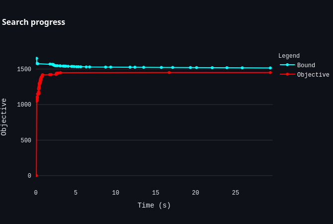 |
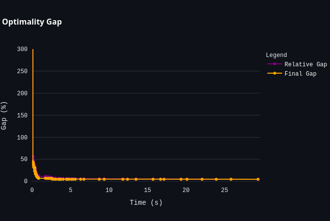 |
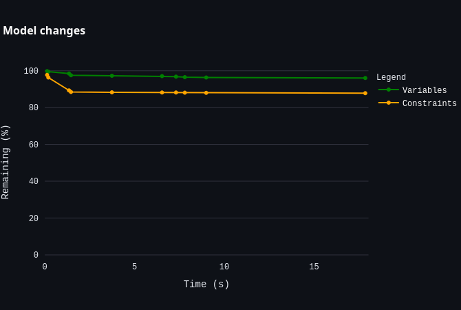 |
|---|---|---|
| Shows how the lower and upper bounds change over time. | Shows how quickly the optimality gap converges. | Shows how the model changes over time as new insights from the search allow the solver to fix variables. |
Subsolver Details
Now there comes a lot of information about the different subsolvers that are used. This is a very detailed part of the log and can be overwhelming. You already need to be rather deep into the details of CP-SAT to actually make any use of this information. It is primarily intended for the developers of CP-SAT. It gives you insights into how the various subsolvers have been contributing to the solution, how the otherwise hidden LP-techniques, including cutting planes, have been used, and how the different heuristics have been applied. Based on this data, you could try to tune the various parameters of CP-SAT for your problem. However, note that you will probably need a lot of experience and experiments to gain an advantage compared to the default settings.
Task timing                          n [     min,      max]      avg      dev     time         n [     min,      max]      avg      dev    dtime
                     'core':         1 [  29.95s,   29.95s]   29.95s   0.00ns   29.95s         1 [  27.99s,   27.99s]   27.99s   0.00ns   27.99s
               'default_lp':         1 [  29.94s,   29.94s]   29.94s   0.00ns   29.94s         1 [  21.11s,   21.11s]   21.11s   0.00ns   21.11s
         'feasibility_pump':       123 [  4.51ms,  70.61ms]  38.93ms   9.87ms    4.79s       122 [  6.31ms,  41.77ms]  17.96ms   6.53ms    2.19s
          'fj_long_default':         1 [ 10.28ms,  10.28ms]  10.28ms   0.00ns  10.28ms         1 [  2.08ms,   2.08ms]   2.08ms   0.00ns   2.08ms
         'fj_short_default':         1 [579.83us, 579.83us] 579.83us   0.00ns 579.83us         0 [  0.00ns,   0.00ns]   0.00ns   0.00ns   0.00ns
                'fs_random':         1 [  6.57ms,   6.57ms]   6.57ms   0.00ns   6.57ms         1 [ 20.00ns,  20.00ns]  20.00ns   0.00ns  20.00ns
  'fs_random_quick_restart':         1 [  6.82ms,   6.82ms]   6.82ms   0.00ns   6.82ms         1 [ 20.00ns,  20.00ns]  20.00ns   0.00ns  20.00ns
            'graph_arc_lns':       123 [  3.65ms, 430.55ms] 169.44ms 106.16ms   20.84s       123 [ 10.00ns, 119.31ms]  61.95ms  43.70ms    7.62s

...

Clauses shared            Num
                 'core':  137
           'default_lp':    1
       'lb_tree_search':    4
               'max_lp':    1
                'no_lp':   10
  'objective_lb_search':    3
         'pseudo_costs':    4
        'quick_restart':    4
  'quick_restart_no_lp':   74
        'reduced_costs':    2
Summary
This final block of the log contains a summary by the solver. Here you find the most important information, such as how successful the search was.
You can find the original documentation here.
CpSolverResponse summary:
status: FEASIBLE  # The status of the search. Can be FEASIBLE, OPTIMAL, INFEASIBLE, UNKNOWN, or MODEL_INVALID.
objective: 1450  # The value of the objective function for the best solution found.
best_bound: 1515  # The proven bound on the objective function, i.e., the best possible value.
integers: 416
booleans: 857
conflicts: 0
branches: 370
propagations: 13193
integer_propagations: 6897
restarts: 370
lp_iterations: 0
walltime: 30.4515  # The time in seconds since solver creation.
usertime: 30.4515
deterministic_time: 306.548
gap_integral: 1292.47  # The integral of the gap over time. A lower value will indicate that the solver is converging faster.
solution_fingerprint: 0xf10c47f1901c2c16  # Useful to check if two runs result in the same solution.
How does it work?
CP-SAT is a versatile portfolio solver, centered around a Lazy Clause Generation (LCG) based Constraint Programming Solver, although it encompasses a broader spectrum of technologies.
In its role as a portfolio solver, CP-SAT concurrently executes a multitude of diverse algorithms and strategies, each possessing unique strengths and weaknesses. These elements operate largely independently but engage in information exchange, sharing progress when better solutions emerge or tighter bounds become available.
While this may initially appear as an inefficient approach due to potential redundancy, it proves highly effective in practice. The rationale behind this lies in the inherent challenge of predicting which algorithm is best suited to solve a given problem (No Free Lunch Theorem). Thus, the pragmatic strategy involves running various approaches in parallel, with the hope that one will effectively address the problem at hand. Note that you can also specify which algorithms should be used if you already know which strategies are promising or futile.
In contrast, Branch and Cut-based Mixed Integer Programming solvers like Gurobi implement a more efficient partitioning of the search space to reduce redundancy. However, they specialize in a particular strategy, which may not always be the optimal choice, although it frequently proves to be so.
CP-SAT employs Branch and Cut techniques, including linear relaxations and cutting planes, as part of its toolkit. Models that can be efficiently addressed by a Mixed Integer Programming (MIP) solver are typically a good match for CP-SAT as well. Nevertheless, CP-SAT's central focus is the implementation of Lazy Clause Generation, harnessing SAT-solvers rather than relying primarily on linear relaxations. As a result, CP-SAT may exhibit somewhat reduced performance when confronted with MIP problems compared to dedicated MIP solvers. However, it gains a distinct advantage when dealing with problems laden with intricate logical constraints.
The concept behind Lazy Clause Generation involves the (incremental) transformation of the problem into a SAT-formula, subsequently employing a SAT-solver to seek a solution (or prove bounds by infeasibility). To mitigate the impracticality of a straightforward conversion, Lazy Clause Generation leverages an abundance of lazy variables and clauses.
Notably, the Cook-Levin Theorem attests that any problem within the realm of NP can be translated into a SAT-formula. Optimization, in theory, could be achieved through a simple binary search. However, this approach, while theoretically sound, lacks efficiency. CP-SAT employs a more refined encoding scheme to tackle optimization problems more effectively.
If you want to understand the inner workings of CP-SAT, you can follow the following learning path:
- Learn how to get a feasible solution based on boolean logics with SAT-solvers: Backtracking, DPLL, CDCL, VSIDS, ...
- Learn how to get provably optimal solutions via classical Mixed Integer
Programming:
- Linear Programming: Simplex, Duality, Dual Simplex, ...
- Understanding and Using Linear Programming (book)
- Optimization in Operations Research by Ronald Rardin (very long book also containing Mixed Integer Programming, Heuristics, and advanced topics. For those who want to dive deep.)
- Video Series by Gurobi
- Mixed Integer Programming: Branch and Bound, Cutting Planes, Branch and
Cut, ...
- Discrete Optimization on Coursera with Pascal Van Hentenryck and Carleton Coffrin (video course, including also Constraint Programming and Heuristics)
- Gurobi Resources (website)
- Linear Programming: Simplex, Duality, Dual Simplex, ...
- Learn the additional concepts of LCG Constraint Programming: Propagation, Lazy Clause Generation, ...
- Learn the details of CP-SAT:
- The proto-file of the parameters (source)
- The complete source code (source)
- A recent talk by the developers of CP-SAT (video)
- Another recent talk by the developers of CP-SAT (video)
- A talk by the developers of CP-SAT (video)
If you already have a background in Mixed Integer Programming, you may directly jump into the slides of Combinatorial Optimisation and Constraint Programming. This is a full and detailed course on constraint programming, and will probably take you some time to work through. However, it gives you all the knowledge you need to understand the constraint programming part of CP-SAT.
Originally, I wrote a short introduction into each of the topics, but I decided to remove them as the material I linked to is much better than what I could have written. You can find a backup of the old version here.
What happens in CP-SAT on solve?
What actually happens when you execute solver.Solve(model)?
- The model is read.
- The model is verified.
- Preprocessing (multiple iterations):
- Presolve (domain reduction) - Check this video for SAT preprocessing, this video for MaxSAT preprocessing, and this paper for MIP presolving.
- Expanding higher-level constraints to lower-level constraints. See also the analogous FlatZinc and Flattening.
- Detection of equivalent variables and affine relations.
- Substitute these by canonical representations
- Probe some variables to detect if they are actually fixed or detect further equivalences.
- Load the preprocessed model into the underlying solver and create the linear relaxations.
- Search for solutions and bounds with the different solvers until the lower and upper bound match or another termination criterion is reached (e.g., time limit)
- Transform solution back to original model.
This is taken from this talk and slightly extended.
The use of linear programming techniques
As already mentioned before, CP-SAT also utilizes the (dual) simplex algorithm and linear relaxations. The linear relaxation is implemented as a propagator and potentially executed at every node in the search tree but only at lowest priority. A significant difference to the application of linear relaxations in branch and bound algorithms is that only some pivot iterations are performed (to make it faster). However, as there are likely much deeper search trees and the warm-starts are utilized, the optimal linear relaxation may still be computed, just deeper down the tree (note that for SAT-solving, the search tree is usually traversed DFS). At root level, even cutting planes such as Gomory-Cuts are applied to improve the linear relaxation.
The linear relaxation is used for detecting infeasibility (IPs can actually be more powerful than simple SAT, at least in theory), finding better bounds for the objective and variables, and also for making branching decisions (using the linear relaxation's objective and the reduced costs).
The used Relaxation Induced Neighborhood Search RINS (LNS worker), a very successful heuristic, of course also uses linear programming.
Limitations of CP-SAT
While CP-SAT is undeniably a potent solver, it does possess certain limitations when juxtaposed with alternative techniques:
- While proficient, it may not match the speed of a dedicated SAT-solver when tasked with solving SAT-formulas, although its performance remains quite commendable.
- Similarly, for classical MIP-problems, CP-SAT may not outpace dedicated MIP-solvers in terms of speed, although it still delivers respectable performance.
- Unlike MIP/LP-solvers, CP-SAT lacks support for continuous variables, and the workarounds to incorporate them may not always be highly efficient. In cases where your problem predominantly features continuous variables and linear constraints, opting for an LP-solver is likely to yield significantly improved performance.
- CP-SAT does not offer support for lazy constraints or iterative model building, a feature available in MIP/LP-solvers and select SAT-solvers. Consequently, the application of exponential-sized models, which are common and pivotal in Mixed Integer Programming, may be restricted.
- CP-SAT is limited to the Simplex algorithm and does not feature interior point methods. This limitation prevents it from employing polynomial time algorithms for certain classes of quadratic constraints, such as Second Order Cone constraints. In contrast, solvers like Gurobi utilize the Barrier algorithm to efficiently tackle these constraints in polynomial time.
CP-SAT might also exhibit inefficiency when confronted with certain constraints, such as modulo constraints. However, it's noteworthy that I am not aware of any alternative solver capable of efficiently addressing these specific constraints. At times, NP-hard problems inherently pose formidable challenges, leaving us with no alternative but to seek more manageable modeling approaches instead of looking for better solvers.
Alternatives: CP-SAT's Place in the World of Optimization
When you begin exploring optimization, you will encounter a plethora of tools, techniques, and communities. It can be overwhelming, as these groups, while sharing many similarities, also differ significantly. They might use the same terminology for different concepts or different terms for the same concepts, adding to the confusion. Not too many experts can effectively navigate these varied communities and techniques. Often, even specialists, including professors, concentrate on a singular technique or community, remaining unaware of potentially more efficient methods developed in other circles.
If you are interested in understanding the connections between different optimization concepts, consider watching the talk Logic, Optimization, and Constraint Programming: A Fruitful Collaboration by John Hooker. Please note that this is an academic presentation and assumes some familiarity with theoretical computer science.
Let us now explore the various tools and techniques available, and see how they compare to CP-SAT. Please note that this overview is high-level and not exhaustive. If you have any significant additions, feel free to open an issue, and I will consider including them.
- Mixed Integer (Linear) Programming (MIP): MIP is a highly effective method
for solving a variety of optimization problems, particularly those involving
networks like flow or tour problems. While MIP only supports linear
constraints, making it less expressive than CP-SAT, it is often the best
choice if your model is compatible with these constraints. CP-SAT incorporates
techniques from MIP, but with limitations, including the absence of continuous
variables and incremental modeling. Consequently, pure MIP-solvers, being more
specialized, tend to offer greater efficiency for certain applications.
Notable MIP-solvers include:
- Gurobi: A commercial solver known for its state-of-the-art capabilities in MIP-solving. It offers free academic licenses, exceptional performance, user-friendliness, and comprehensive support through documentation and expert-led webinars. Gurobi is particularly impressive in handling complex, large-scale problems.
- SCIP: An open-source solver that provides a Python interface. Although not as efficient or user-friendly as Gurobi, SCIP allows extensive customization and is ideal for research and development, especially for experts needing to implement advanced decomposition techniques.
- HiGHS: A newer solver licensed under MIT, presenting an interesting alternative to SCIP. It is possibly faster and features a more user-friendly interface, but is less versatile. For performance benchmarks, see here.
- Constraint Programming (CP): Constraint Programming is a more general
approach to optimization problems than MIP. As the name suggests, it focuses
on constraints and solvers usually come with a lot of advanced constraints
that can be used to describe your problem more naturally. A classical example
is the
AllDifferent-constraint, which is very hard to model in MIP, but would allow, e.g., to trivially model a Sudoku problem. Constraint Programming has been very successful for example in solving scheduling problems, where you have a lot of constraints that are hard to model with linear constraints. The internal techniques of CP-solvers are often more logic-based and less linear algebra-based than MIP-solvers. Popular CP-solvers are:- OR-Tools' CP-SAT: Discussed in this primer, CP-SAT combines various optimization techniques, including those from MIP solvers, but its primary technique is Lazy Clause Generation. This approach translates problems into (Max-)SAT formulas for resolution.
- Choco: A traditional CP solver developed in Java, licensed under the BSD 4-Clause. While it may not match CP-SAT in efficiency or modernity, Choco offers significant flexibility, including the option to integrate custom propagators.
- SAT-Solvers: If your problem is actually just to find a feasible solution
for some boolean variables, you may want to use a SAT-solver. SAT-solvers are
surprisingly efficient and can often handle problems with millions of
variables. If you are clever, you can also do some optimization problems with
SAT-solvers, as CP-SAT actually does. Most SAT-solvers support incremental
modelling, and some support cardinality constraints. However, they are pretty
low-level and CP-SAT actually can achieve similar performance for many
problems. A popular library for SAT-solvers is:
- PySAT: PySAT is a Python library under MIT license that provides a nice interface to many SAT-solvers. It is very easy to use and allows you to switch between different solvers without changing your code. It is a good choice if you want to experiment with SAT-solvers.
- There are many solvers popping up every year and many of them are open source. Check out the SAT Competition to see the current state of the art. Most of the solvers are written in C or C++ and do not provide much documentation. However, as SAT-formulas are very simple and the solvers usually do not have complex dependencies, they can still be reasonably easy to use.
- Satisfiability modulo theories (SMT): SMT-solvers represent an advanced
tier above traditional SAT-solvers. They aim to check the satisfiability of
mathematical formulas by extending propositional logic with additional
theories like linear arithmetic, bit-vectors, arrays, and quantifiers. For
instance, an SMT-solver can determine if a formula is satisfiable under
conditions where all variables are integers that meet specific linear
constraints. Similar to the Lazy Clause Generation utilized by CP-SAT,
SMT-solvers usually use a SAT-solver in the backend, extended by complex
encodings and additional propagators to handle an extensive portfolio of
expressions. These solvers are commonly used in automated theorem proving and
system verification. A popular SMT-solver is:
- Z3: Developed by Microsoft and available under the MIT license, Z3 offers a robust Python interface and comprehensive documentation, making it accessible for a variety of applications.
- Nonlinear Programming (NLP): Many MIP-solvers can actually handle some
nonlinear constraints, as people noticed that some techniques are actually
more general than just for linear constraints, e.g., interior points methods
can also solve second-order cone problems. However, you will notice serious
performance downgrades. If your constraints and objectives get too complex,
they may also no longer be a viable option. If you have smaller optimization
problems of (nearly) any kind, you may want to look into:
- SciPy: SciPy is a Python library that offers a wide range of optimization algorithms. Do not expect it to get anywhere near the performance of a specialized solver, but it gives you a bunch of different options to solve a multitude of problems.
- Modeling Languages: Modeling languages provide a high-level, user-friendly
interface for formulating optimization problems, focusing on the challenges of
developing and maintaining models that accurately reflect real-world
scenarios. These languages are solver-agnostic, allowing easy switching
between different solvers - such as from the free SCIP solver to the
commercial Gurobi - without modifying the underlying model. They also
facilitate the use of diverse techniques, like transitioning between
constraint programming and mixed integer programming. However, the trade-off
is a potential loss of control and performance for the sake of generality and
simplicity. Some of the most popular modeling languages include:
- MiniZinc: Very well-documented and free modelling language that seems to have a high reputation especially in the academic community. The amazing course on constraint programming by Pierre Flener also uses MiniZinc. It supports many backends and there are the MiniZinc Challenges, where CP-SAT won quite a lot of medals.
- AMPL: AMPL is possibly the most popular modelling language. It has free and commercial solvers. There is not only extensive documentation, but even a book on how to use it.
- GAMS: This is a commercial system which supports many solvers and also has gotten a Python-interface. I actually know the guys from GAMS as they have a location in Braunschweig. They have a lot of experience in optimization, but I have never used their software myself.
- pyomo: Pyomo is a Python library that allows you to model your optimization problem in Python and then let it solve by different solvers. It is not as high-level as AMPL or GAMS, but it is free and open source. It is also very flexible and allows you to use Python to model your problem, which is a huge advantage if you are already familiar with Python. It actually has support for CP-SAT and could be an option if you just want to have a quick solution.
- OR-Tools' MathOpt: A very new competitor and sibling of CP-SAT. It only supports a few solvers, but may be still interesting.
- Specialized Algorithms: For many optimization problems, there are
specialized algorithms that can be much more efficient than general-purpose
solvers. Examples are:
- Concorde: Concorde is a solver for the Traveling Salesman Problem that despite its age is still blazingly fast for many instances.
- OR-Tools' Routing Solver: OR-Tools also comes with a dedicated solver for routing problems.
- OR-Tools' Network Flows: OR-Tools also comes with a dedicated solver for network flow problems.
- ...
- Approximation Algorithms: For many difficult optimization problems, you can find scientific papers that describe approximation algorithms for them. These algorithms come with some guarantees of not being too far off from the optimal solution. Some are even proven to achieve the best possible guarantees. However, you should not directly try to implement such a paper even if it perfectly fits your problem. There are some approximation algorithms that are actually practical, but many are not. The guarantees are usually focussed on artificial worst-case scenarios, and even if the algorithms can be implemented, they may be beaten by simple heuristics. Approximation algorithms and their analysis can be quite useful for understanding the structure of your problem, but their direct practical use is limited.
- Meta-Heuristics: Instead of using a generic solver like CP-SAT, you can also try to build a custom algorithm for your problem based on some meta-heuristic pattern, like simulated annealing, genetic algorithms, or tabu search. Meta-heuristics require some coding, but once you know the pattern, they are quite straightforward to implement. While there are some libraries to generalize parts of the algorithms, you could also just write the whole algorithm yourself. This gives the advantage of truly understanding what is going on in the algorithm, but you miss a lot of advanced techniques contained in solvers like CP-SAT. For many optimization problems, you will have difficulties competing against techniques utilizing advanced solvers in terms of solution quality. If you just want a quick solution, meta-heuristics can be a good start.
As evident, there exists a diverse array of tools and techniques for solving optimization problems. CP-SAT stands out as a versatile approach, particularly well-suited for combinatorial optimization challenges. If you frequently encounter these types of problems, becoming proficient with CP-SAT is highly recommended. Its effectiveness across a broad spectrum of scenarios - excelling in many - is remarkable for a tool that is both free and open-source.
Part 2: Advanced Topics
Coding Patterns for Optimization Problems
In this section, we will explore various coding patterns that are essential for structuring implementations for optimization problems using CP-SAT. While we will not delve into the modeling of specific problems, our focus will be on demonstrating how to organize your code to enhance its readability and maintainability. These practices are crucial for developing robust and scalable optimization solutions that can be easily understood, modified, and extended by other developers. We will concentrate on basic patterns, as more complex patterns are better understood within the context of larger problems and are beyond the scope of this primer.
[!WARNING]
The naming conventions for patterns in optimization problems are not standardized. There is no comprehensive guide on coding patterns for optimization issues, and my insights are primarily based on personal experience. Most online examples tend to focus solely on the model, often presented as Jupyter notebooks or sequential scripts. The gurobi-optimods provide the closest examples to production-ready code that I am aware of, yet they offer limited guidance on code structuring. I aim to address this gap, which many find challenging, though it is important to note that my approach is highly opinionated.
Simple Function
For straightforward optimization problems, encapsulating the model creation and solving within a single function is a practical approach. This method is best suited for simpler cases due to its straightforward nature but lacks flexibility for more complex scenarios. Parameters such as the time limit and optimality tolerance can be customized via keyword arguments with default values.
The following Python function demonstrates solving a simple knapsack problem using CP-SAT. To recap, in the knapsack problem, we select items - each with a specific weight and value - to maximize total value without exceeding a predefined weight limit. Given its simplicity, involving only one constraint, the knapsack problem serves as an ideal model for introductory examples.
from ortools.sat.python import cp_model
from typing import List

def solve_knapsack(
    weights: List[int],
    values: List[int],
    capacity: int,
    *,
    time_limit: int = 900,
    opt_tol: float = 0.01,
) -> List[int]:
    # initialize the model
    model = cp_model.CpModel()
    n = len(weights)  # Number of items
    # Decision variables for items
    x = [model.new_bool_var(f"x_{i}") for i in range(n)]
    # Capacity constraint
    model.add(sum(weights[i] * x[i] for i in range(n)) <= capacity)
    # Objective function to maximize value
    model.maximize(sum(values[i] * x[i] for i in range(n)))
    # Solve the model
    solver = cp_model.CpSolver()
    solver.parameters.max_time_in_seconds = time_limit  # Solver time limit
    solver.parameters.relative_gap_limit = opt_tol  # Solver optimality tolerance
    status = solver.solve(model)
    # Extract solution
    return (
        # Return indices of selected items
        [i for i in range(n) if solver.value(x[i])]
        if status in [cp_model.OPTIMAL, cp_model.FEASIBLE]
        else []
    )
Logging the Model Building
When working with more complex optimization problems, logging the model-building process can be essential to find and fix issues. Often, the problem lies not within the solver but in the model itself.
In the following example, we add some basic logging to the solver function to give us some insights into the model-building process. This logging can be easily activated or deactivated by the logging framework, allowing us to use it not only during development but also in production.
If you do not know about the logging framework of Python, this is an excellent moment to learn about it. I consider it an essential skill for production code and this and similar frameworks are used for most production code in any language. The official Python documentation contains a good tutorial.
import logging
from ortools.sat.python import cp_model
from typing import List

_logger = logging.getLogger(__name__)  # get a logger for the current module

def solve_knapsack(
    weights: List[int],
    values: List[int],
    capacity: int,
    *,
    time_limit: int = 900,
    opt_tol: float = 0.01,
) -> List[int]:
    _logger.debug("Building the knapsack model")
    # initialize the model
    model = cp_model.CpModel()
    n = len(weights)  # Number of items
    _logger.debug("Number of items: %d", n)
    if n > 0:
        _logger.debug(
            "Min/Mean/Max weight: %d/%.2f/%d",
            min(weights),
            sum(weights) / n,
            max(weights),
        )
        _logger.debug(
            "Min/Mean/Max value: %d/%.2f/%d", min(values), sum(values) / n, max(values)
        )
    # Decision variables for items
    x = [model.new_bool_var(f"x_{i}") for i in range(n)]
    # Capacity constraint
    model.add(sum(weights[i] * x[i] for i in range(n)) <= capacity)
    # Objective function to maximize value
    model.maximize(sum(values[i] * x[i] for i in range(n)))
    # Log the model
    _logger.debug("Model created with %d items", n)
    # Solve the model
    solver = cp_model.CpSolver()
    solver.parameters.max_time_in_seconds = time_limit  # Solver time limit
    solver.parameters.relative_gap_limit = opt_tol  # Solver optimality tolerance
    _logger.debug(
        "Starting the solution process with time limit %d seconds", time_limit
    )
    status = solver.solve(model)
    # Extract solution
    selected_items = (
        [i for i in range(n) if solver.value(x[i])]
        if status in [cp_model.OPTIMAL, cp_model.FEASIBLE]
        else []
    )
    _logger.debug("Selected items: %s", selected_items)
    return selected_items
We will not use logging in the following examples to save space, but you should consider adding it to your code.
[!TIP]
A great hack you can do with the logging framework is that you can easily hook into your code and do analysis beyond the simple logging. You can simply write a handler that, e.g., waits for the tag
"Selected items: %s"and then can directly access the selected items, as the actual object is passed to the handler (and not just the string). This can be very useful to gather statistics or to visualize the search process, without having to change the (production) code.
Custom Data Classes for Instances, Configurations, and Solutions
Incorporating serializable data classes to manage instances, configurations, and solutions significantly enhances the readability and maintainability of your code. These classes also facilitate the documentation process, testing, and ensure data consistency across larger projects where data exchange among different components is necessary.
Implemented Changes: We introduce data classes using Pydantic, a popular Python library that supports data validation and settings management through Python type annotations. The changes include:
- Instance Class: Defines the knapsack problem with attributes for weights, values, and capacity. It includes a validation method to ensure that the number of weights matches the number of values, thereby enhancing data integrity.
- Configuration Class: Manages solver settings such as time limits and optimality tolerance, allowing for easy adjustments and fine-tuning of the solver’s performance. Default values ensure backward compatibility, facilitating the seamless integration of older configurations with new parameters.
- Solution Class: Captures the outcome of the optimization process, including which items were selected, the objective value, and the upper bound of the solution. This class allows us to add additional information, instead of just returning the pure solution. It also allows us to later extend the attached information without breaking the API, by just making the new entries optional or providing a default value. For example, you may be interested in the solution time that was required to find the solution.
from ortools.sat.python import cp_model
from pydantic import BaseModel, PositiveInt, NonNegativeFloat

class KnapsackInstance(BaseModel):
    weights: list[PositiveInt]  # the weight of each item
    values: list[PositiveInt]  # the value of each item
    capacity: PositiveInt  # the capacity of the knapsack

    @model_validator(mode="after")
    def check_lengths(cls, v):
        if len(v.weights) != len(v.values):
            raise ValueError("Mismatch in number of weights and values.")
        return v

class KnapsackSolverConfig(BaseModel):
    time_limit: PositiveInt = 900  # Solver time limit in seconds
    opt_tol: NonNegativeFloat = 0.01  # Optimality tolerance (1% gap allowed)
    log_search_progress: bool = False  # Whether to log search progress

class KnapsackSolution(BaseModel):
    selected_items: list[int]  # Indices of the selected items
    objective: float  # Objective value of the solution
    upper_bound: float  # Upper bound of the solution

def solve_knapsack(
    instance: KnapsackInstance, config: KnapsackSolverConfig
) -> KnapsackSolution:
    model = cp_model.CpModel()
    n = len(instance.weights)
    x = [model.new_bool_var(f"x_{i}") for i in range(n)]
    model.add(sum(instance.weights[i] * x[i] for i in range(n)) <= instance.capacity)
    model.maximize(sum(instance.values[i] * x[i] for i in range(n)))
    solver = cp_model.CpSolver()
    # Set solver parameters from the configuration
    solver.parameters.max_time_in_seconds = config.time_limit
    solver.parameters.relative_gap_limit = config.opt_tol
    solver.parameters.log_search_progress = config.log_search_progress
    # solve the model and return the solution
    status = solver.solve(model)
    if status in [cp_model.OPTIMAL, cp_model.FEASIBLE]:
        return KnapsackSolution(
            selected_items=[i for i in range(n) if solver.value(x[i])],
            objective=solver.objective_value,
            upper_bound=solver.best_objective_bound,
        )
    return KnapsackSolution(selected_items=[], objective=0, upper_bound=0)
Key Benefits:
- Structured Data Handling: Defining explicit structures for each aspect of the problem ensures robust data handling and minimizes errors, facilitating easier integration and API exposition.
- Easy Serialization: Pydantic models support straightforward conversion to and from JSON, simplifying the storage and transmission of configurations and results.
- Enhanced Testing and Documentation: Clear data definitions make it easier to generate documentation and conduct tests that confirm the model and solver's behavior.
- Backward Compatibility: Default values in data classes enable seamless integration of older configurations with new software versions, accommodating new parameters without disrupting existing setups.
- Type Hinting: Type annotations in data classes provide a clear specification of the expected data types, enhancing code readability and enabling static type checkers to catch potential errors early.
[!TIP]
One challenge I often face is designing data classes to be as generic as possible so that they can be used with multiple solvers and remain compatible throughout various stages of the optimization process. For instance, a graph might be represented as an edge list, an adjacency matrix, or an adjacency list, each with its own pros and cons, complicating the decision of which format is optimal for all stages. However, converting between different data class formats is typically straightforward, often requiring only a few lines of code and having a negligible impact compared to the optimization process itself. Therefore, I recommend focusing on functionality with your current solver without overcomplicating this aspect. There is little harm in having to call a few convert functions because you created separate specialized data classes.
Solver Class
In many real-world optimization scenarios, problems may require iterative refinement of the model and solution. For instance, new constraints might only become apparent after presenting an initial solution to a user or another algorithm. In such cases, flexibility is crucial, making it beneficial to encapsulate both the model and the solver within a single class. This setup facilitates the dynamic addition of constraints and subsequent re-solving without needing to rebuild the entire model.
Implemented Changes: We introduce the KnapsackSolver class, which
encapsulates the entire setup and solving process of the knapsack problem:
class KnapsackSolver:
    def __init__(self, instance: KnapsackInstance, config: KnapsackSolverConfig):
        self.instance = instance
        self.config = config
        self.model = cp_model.CpModel()
        self.n = len(instance.weights)
        self.x = [self.model.new_bool_var(f"x_{i}") for i in range(self.n)]
        self._build_model()
        self.solver = cp_model.CpSolver()

    def _add_constraints(self):
        used_weight = sum(
            weight * x_i for weight, x_i in zip(self.instance.weights, self.x)
        )
        self.model.add(used_weight <= self.instance.capacity)

    def _add_objective(self):
        self.model.maximize(
            sum(value * x_i for value, x_i in zip(self.instance.values, self.x))
        )

    def _build_model(self):
        self._add_constraints()
        self._add_objective()

    def solve(self) -> KnapsackSolution:
        self.solver.parameters.max_time_in_seconds = self.config.time_limit
        self.solver.parameters.relative_gap_limit = self.config.opt_tol
        self.solver.parameters.log_search_progress = self.config.log_search_progress
        status = self.solver.solve(self.model)
        if status in [cp_model.OPTIMAL, cp_model.FEASIBLE]:
            return KnapsackSolution(
                selected_items=[
                    i for i in range(self.n) if self.solver.value(self.x[i])
                ],
                objective=self.solver.objective_value,
                upper_bound=self.solver.best_objective_bound,
            )
        return KnapsackSolution(
            selected_items=[], objective=0, upper_bound=float("inf")
        )

    def prohibit_combination(self, item_a: int, item_b: int):
        """
        Prohibit the combination of two items in the solution,
        without having to know the actual model, e.g., if they
        do not follow clean rules but after presenting the solution
        to the user, the user decides that these two items should
        not be packed together. After calling this method, you can
        simply call `solve` again to get a new solution obeying
        this constraint.
        """
        self.model.add(self.x[item_a] + self.x[item_b] <= 1)

if __name__ == "__main__":
    instance = KnapsackInstance(weights=[1, 2, 3], values=[4, 5, 6], capacity=3)
    config = KnapsackSolverConfig(time_limit=10, opt_tol=0.01, log_search_progress=True)
    solver = KnapsackSolver(instance, config)
    solution = solver.solve()
    print(solution)
    solver.prohibit_combination(0, 1)
    solution = solver.solve()
    print(solution)
Key Benefits:
- Incremental Model Building and Re-solving: The class structure not only
facilitates incremental additions of constraints for iterative model
modifications without starting from scratch but also supports multiple
invocations of the
solvemethod. This allows for iterative refinement of the solution by adjusting constraints or solver parameters such as time limits and optimality tolerance. - Direct Model and Solver Access: Provides direct member-access to the model and solver, enhancing flexibility for advanced operations and debugging, a capability not exposed in the function-based approach.
Exchangeable Objective
In real-world scenarios, objectives are often not clearly defined. Typically, there are multiple objectives with different priorities, making it challenging to combine them. Consider the Knapsack problem, representing a logistics issue where we aim to transport the maximum value of goods in a single trip. Given the values and weights of the goods, our primary objective is to maximize the packed goods' value. However, after computing and presenting the solution, we might be asked to find an alternative solution that does not fill the truck as much, even if it means accepting up to a 5% decrease in value.
To handle this, we can optimize in two phases. First, we maximize the value under the weight constraint. Next, we add a constraint that the value must be at least 95% of the initial solution's value and change the objective to minimize the weight. This iterative process can continue through multiple phases, exploring the Pareto front of the two objectives. More complex problems can be tackled using similar approaches.
A challenge with this method is avoiding the creation of multiple models and restarting from scratch in each phase. Since we have a solution close to the new one, we can use it as a starting point. This technique, known as warm-starting, is common in optimization and significantly reduces the time needed to find a solution. Additionally, reusing the model can improve code readability and performance.
The following code demonstrates how to extend a solver class to support exchangeable objectives. It includes fixing the current objective value to prevent degeneration and using the current solution as a hint.
Implemented Changes: We created a member _objective to store the current
objective function and added methods to set the objective to maximize value or
minimize weight. We also introduced methods to set the solution as a hint for
the next solve which will automatically be called if the solve found a
feasible solution. To not degenerate on previous objectives, we added a method
to fix the current objective value based on some ratio.
class MultiObjectiveKnapsackSolver:
    def __init__(self, instance: KnapsackInstance, config: KnapsackSolverConfig):
        self.instance = instance
        self.config = config
        self.model = cp_model.CpModel()
        self.n = len(instance.weights)
        self.x = [self.model.new_bool_var(f"x_{i}") for i in range(self.n)]
        self._objective = 0
        self._build_model()
        self.solver = cp_model.CpSolver()

    def set_maximize_value_objective(self):
        """Set the objective to maximize the value of the packed goods."""
        self._objective = sum(
            value * x_i for value, x_i in zip(self.instance.values, self.x)
        )
        self.model.maximize(self._objective)

    def set_minimize_weight_objective(self):
        """Set the objective to minimize the weight of the packed goods."""
        self._objective = sum(
            weight * x_i for weight, x_i in zip(self.instance.weights, self.x)
        )
        self.model.minimize(self._objective)

    def _set_solution_as_hint(self):
        """Use the current solution as a hint for the next solve."""
        for i, v in enumerate(self.model.proto.variables):
            v_ = self.model.get_int_var_from_proto_index(i)
            assert v.name == v_.name, "Variable names should match"
            self.model.add_hint(v_, self.solver.value(v_))

    def fix_current_objective(self, ratio: float = 1.0):
        """Fix the current objective value to prevent degeneration."""
        if ratio == 1.0:
            self.model.add(self._objective == self.solver.objective_value)
        elif ratio > 1.0:
            self.model.add(self._objective <= ceil(self.solver.objective_value * ratio))
        else:
            self.model.add(
                self._objective >= floor(self.solver.objective_value * ratio)
            )

    def _add_constraints(self):
        """Add the weight constraint to the model."""
        used_weight = sum(
            weight * x_i for weight, x_i in zip(self.instance.weights, self.x)
        )
        self.model.add(used_weight <= self.instance.capacity)

    def _build_model(self):
        """Build the initial model with constraints and objective."""
        self._add_constraints()
        self.set_maximize_value_objective()

    def solve(self) -> KnapsackSolution:
        """Solve the knapsack problem and return the solution."""
        self.solver.parameters.max_time_in_seconds = self.config.time_limit
        self.solver.parameters.relative_gap_limit = self.config.opt_tol
        self.solver.parameters.log_search_progress = self.config.log_search_progress
        status = self.solver.solve(self.model)
        if status in [cp_model.OPTIMAL, cp_model.FEASIBLE]:
            self._set_solution_as_hint()
            return KnapsackSolution(
                selected_items=[
                    i for i in range(self.n) if self.solver.value(self.x[i])
                ],
                objective=self.solver.objective_value,
                upper_bound=self.solver.best_objective_bound,
            )
        return KnapsackSolution(
            selected_items=[], objective=0, upper_bound=float("inf")
        )
We can use the MultiObjectiveKnapsackSolver class as follows:
config = KnapsackSolverConfig(time_limit=15, opt_tol=0.01, log_search_progress=True)
solver = MultiObjectiveKnapsackSolver(instance, config)
solution_1 = solver.solve()

# maintain at least 95% of the current objective value
solver.fix_current_objective(0.95)
# change the objective to minimize the weight
solver.set_minimize_weight_objective()
solution_2 = solver.solve()
Key Benefits:
- Objective Flexibility: The ability to exchange objectives and fix the current objective value enhances the solver's adaptability to changing requirements and constraints, enabling the exploration of multiple objectives and trade-offs.
- Warm-Starting: By using the current solution as a hint for the next solve, the solver can leverage the existing solution to find a new one more quickly, reducing computational overhead and improving performance.
Variable Containers
In complex models, variables play a crucial role and can span the entire model. While managing variables as a list or dictionary may suffice for simple models, this approach becomes cumbersome and error-prone as the model's complexity increases. A single mistake in indexing can introduce subtle errors, potentially leading to incorrect results that are difficult to trace.
As variables form the foundation of the model, refactoring them becomes more challenging as the model grows. Therefore, it is crucial to establish a robust management system early on. Encapsulating variables in a dedicated class ensures that they are always accessed correctly. This approach also allows for the easy addition of new variables or modifications in their management without altering the entire model.
Furthermore, incorporating clear query methods helps maintain the readability and manageability of constraints. Readable constraints, free from complex variable access patterns, ensure that the constraints accurately reflect the intended model.
Implemented Changes: We introduce the _ItemVariables class to the
KnapsackSolver, which acts as a container for the decision variables
associated with the knapsack items. This class not only creates these variables
but also offers several utility methods to interact with them, improving the
clarity and maintainability of the code.
from typing import Generator, Tuple

class _ItemVariables:
    def __init__(self, instance: KnapsackInstance, model: cp_model.CpModel):
        self.instance = instance
        self.x = [model.new_bool_var(f"x_{i}") for i in range(len(instance.weights))]

    def __getitem__(self, i):
        return self.x[i]

    def extract_packed_items(self, solver: cp_model.CpSolver) -> List[int]:
        return [i for i, x_i in enumerate(self.x) if solver.value(x_i)]

    def used_weight(self) -> cp_model.LinearExpr:
        return sum(weight * x_i for weight, x_i in zip(self.instance.weights, self.x))

    def packed_value(self) -> cp_model.LinearExpr:
        return sum(value * x_i for value, x_i in zip(self.instance.values, self.x))

    def iter_items(
        self,
        weight_lb: float = 0.0,
        weight_ub: float = float("inf"),
        value_lb: float = 0.0,
        value_ub: float = float("inf"),
    ) -> Generator[Tuple[int, cp_model.BoolVar], None, None]:
        for i, (weight, x_i) in enumerate(zip(self.instance.weights, self.x)):
            if (
                weight_lb <= weight <= weight_ub
                and value_lb <= self.instance.values[i] <= value_ub
            ):
                yield i, x_i

class KnapsackSolver:
    def __init__(self, instance: KnapsackInstance, config: KnapsackSolverConfig):
        self.instance = instance
        self.config = config
        self.model = cp_model.CpModel()
        self._item_vars = _ItemVariables(instance, self.model)
        self._build_model()
        self.solver = cp_model.CpSolver()

    def _add_constraints(self):
        self.model.add(self._item_vars.used_weight() <= self.instance.capacity)

    def _add_objective(self):
        self.model.maximize(self._item_vars.packed_value())

    def _build_model(self):
        self._add_constraints()
        self._add_objective()

    def solve(self) -> KnapsackSolution:
        self.solver.parameters.max_time_in_seconds = self.config.time_limit
        self.solver.parameters.relative_gap_limit = self.config.opt_tol
        self.solver.parameters.log_search_progress = self.config.log_search_progress
        status = self.solver.solve(self.model)
        if status in [cp_model.OPTIMAL, cp_model.FEASIBLE]:
            return KnapsackSolution(
                selected_items=self._item_vars.extract_packed_items(self.solver),
                objective=self.solver.objective_value,
                upper_bound=self.solver.best_objective_bound,
            )
        return KnapsackSolution(
            selected_items=[], objective=0, upper_bound=float("inf")
        )

    def prohibit_combination(self, item_a: int, item_b: int):
        self.model.add(self._item_vars[item_a] + self._item_vars[item_b] <= 1)
Key Benefits:
- Enhanced Readability: By encapsulating the item variables and their interactions within a dedicated class, the main solver class becomes more focused and easier to understand.
- Improved Modularity: The
_ItemVariables-class allows to easily hand over the variables to a function that may create complex constraints, without creating a cyclic dependency. The model can now be split over multiple files without any issues.
Submodels
As optimization models increase in complexity, it may be beneficial to divide the overall model into smaller, more manageable submodels. These submodels can encapsulate specific parts of the problem, communicating with the main model via shared variables but hiding internal details like auxiliary variables.
For instance, piecewise linear functions can be modeled as submodels, as done
for PiecewiseLinearConstraint in
./utils/piecewise_functions/piecewise_linear_function.py.
Each submodel handles a piecewise linear function independently, interfacing
with the main model through shared x and y variables. By encapsulating the
logic for each piecewise function in a dedicated class, we standardize and reuse
the logic across multiple instances, enhancing modularity and maintainability.
requirements_1 = (3, 5, 2)
requirements_2 = (2, 1, 3)

from ortools.sat.python import cp_model

model = cp_model.CpModel()
buy_1 = model.new_int_var(0, 1_500, "buy_1")
buy_2 = model.new_int_var(0, 1_500, "buy_2")
buy_3 = model.new_int_var(0, 1_500, "buy_3")

produce_1 = model.new_int_var(0, 300, "produce_1")
produce_2 = model.new_int_var(0, 300, "produce_2")

model.add(produce_1 * requirements_1[0] + produce_2 * requirements_2[0] <= buy_1)
model.add(produce_1 * requirements_1[1] + produce_2 * requirements_2[1] <= buy_2)
model.add(produce_1 * requirements_1[2] + produce_2 * requirements_2[2] <= buy_3)

# You can find this code it ./utils!
from piecewise_functions import PiecewiseLinearFunction, PiecewiseLinearConstraint

# Define the functions for the costs
costs_1 = [(0, 0), (1000, 400), (1500, 1300)]
costs_2 = [(0, 0), (300, 300), (700, 500), (1200, 600), (1500, 1100)]
costs_3 = [(0, 0), (200, 400), (500, 700), (1000, 900), (1500, 1500)]
# PiecewiseLinearFunction is a pydantic model and can be serialized easily!
f_costs_1 = PiecewiseLinearFunction(
    xs=[x for x, y in costs_1], ys=[y for x, y in costs_1]
)
f_costs_2 = PiecewiseLinearFunction(
    xs=[x for x, y in costs_2], ys=[y for x, y in costs_2]
)
f_costs_3 = PiecewiseLinearFunction(
    xs=[x for x, y in costs_3], ys=[y for x, y in costs_3]
)

# Define the functions for the gain
gain_1 = [(0, 0), (100, 800), (200, 1600), (300, 2_000)]
gain_2 = [(0, 0), (80, 1_000), (150, 1_300), (200, 1_400), (300, 1_500)]
f_gain_1 = PiecewiseLinearFunction(xs=[x for x, y in gain_1], ys=[y for x, y in gain_1])
f_gain_2 = PiecewiseLinearFunction(xs=[x for x, y in gain_2], ys=[y for x, y in gain_2])

# Create y>=f(x) constraints for the costs
x_costs_1 = PiecewiseLinearConstraint(model, buy_1, f_costs_1, upper_bound=False)
x_costs_2 = PiecewiseLinearConstraint(model, buy_2, f_costs_2, upper_bound=False)
x_costs_3 = PiecewiseLinearConstraint(model, buy_3, f_costs_3, upper_bound=False)

# Create y<=f(x) constraints for the gain
x_gain_1 = PiecewiseLinearConstraint(model, produce_1, f_gain_1, upper_bound=True)
x_gain_2 = PiecewiseLinearConstraint(model, produce_2, f_gain_2, upper_bound=True)

# Maximize the gain minus the costs
model.maximize(x_gain_1.y + x_gain_2.y - (x_costs_1.y + x_costs_2.y + x_costs_3.y))
Key Benefits:
- Testing: Testing complex optimization models is often very difficult as
the outputs are often sensitive to small changes in the model. Even if you
have a good test case with predictable results, detected errors may be very
difficult to track down. If you extracted elements into submodels, you can
test these submodels independently, ensuring that they work correctly before
integrating them into the main model.
def test_piecewise_linear_upper_bound_constraint(): model = cp_model.CpModel() # Defining the input. Note that for some problems it may be # easier to fix variables to a specific value and then just # test feasibility. x = model.new_int_var(0, 20, "x") f = PiecewiseLinearFunction(xs=[0, 10, 20], ys=[0, 10, 5]) # Using the submodel c = PiecewiseLinearConstraint(model, x, f, upper_bound=True) model.maximize(c.y) # Checking its behavior solver = cp_model.CpSolver() assert solver.solve(model) == cp_model.OPTIMAL assert solver.value(c.y) == 10 assert solver.value(x) == 10 - Modularity: Submodels allow for the encapsulation of complex logic into smaller, more manageable components, enhancing code organization and readability.
- Reusability: By defining submodels for common functions or constraints, you can reuse these components across multiple instances of the main model, promoting code reuse and reducing redundancy.
- Abstraction: Submodels abstract the internal details of specific functions, enabling users to interact with them at a higher level without needing to understand the underlying implementation.
Lazy Variable Construction
In models with numerous auxiliary variables, often only a subset is actually used by the constraints. You can now try to only create the variables that may actually be needed later on, but this can require some complex code to ensure that exactly the right variables are created. If the model is extended later on, things can get even more complicated as you may not know which variables are needed upfront. This is where lazy variable construction comes into play. Here, we create variables only when they are accessed, ensuring that only necessary variables are generated, reducing memory usage and computational overhead. While this can be more expensive that just creating a vector with all variables, when in the end most variables are needed anyway, but it can save a lot of memory and computation time if only a small subset is actually used.
Implemented Changes: We introduce the new class _CombiVariables that
manages auxiliary variables indicating that a pair of items were packed,
allowing to give additional bonuses for packing certain items together.
Theoretically, there is a square number of possible combinations, but there will
probably only be a handful of them that are actually used. By creating the
variables only when they are accessed, we can reduce memory usage and
computational overhead.
class _ItemVariables:
    def __init__(self, instance: KnapsackInstance, model: cp_model.CpModel):
        self.instance = instance
        self.x = [model.new_bool_var(f"x_{i}") for i in range(len(instance.weights))]

    def __getitem__(self, i):
        return self.x[i]

    def extract_packed_items(self, solver: cp_model.CpSolver) -> List[int]:
        return [i for i, x_i in enumerate(self.x) if solver.value(x_i)]

    def used_weight(self) -> cp_model.LinearExpr:
        return sum(weight * x_i for weight, x_i in zip(self.instance.weights, self.x))

    def packed_value(self) -> cp_model.LinearExpr:
        return sum(value * x_i for value, x_i in zip(self.instance.values, self.x))

    def iter_items(
        self,
        weight_lb: float = 0.0,
        weight_ub: float = float("inf"),
        value_lb: float = 0.0,
        value_ub: float = float("inf"),
    ) -> Generator[Tuple[int, cp_model.BoolVar], None, None]:
        for i, (weight, x_i) in enumerate(zip(self.instance.weights, self.x)):
            if (
                weight_lb <= weight <= weight_ub
                and value_lb <= self.instance.values[i] <= value_ub
            ):
                yield i, x_i

class _CombiVariables:
    def __init__(
        self,
        instance: KnapsackInstance,
        model: cp_model.CpModel,
        item_vars: _ItemVariables,
    ):
        self.instance = instance
        self.model = model
        self.item_vars = item_vars
        self.bonus = {}

    def __getitem__(self, i, j):
        i, j = min(i, j), max(i, j)
        if (i, j) not in self.bonus:
            self.bonus[(i, j)] = self.model.new_bool_var(f"bonus_{i}_{j}")
            self.model.add(
                self.item_vars[i] + self.item_vars[j] >= 2 * self.bonus[(i, j)]
            )
        return self.bonus[(i, j)]

class KnapsackSolver:
    def __init__(self, instance: KnapsackInstance, config: KnapsackSolverConfig):
        self.instance = instance
        self.config = config
        self.model = cp_model.CpModel()
        self._item_vars = _ItemVariables(instance, self.model)
        self._bonus_vars = _CombiVariables(instance, self.model, self._item_vars)
        self._objective = self._item_vars.packed_value()  # Initial objective setup
        self.solver = cp_model.CpSolver()

    def solve(self) -> KnapsackSolution:
        self.model.maximize(self._objective)
        self.solver.parameters.max_time_in_seconds = self.config.time_limit
        self.solver.parameters.relative_gap_limit = self.config.opt_tol
        self.solver.parameters.log_search_progress = self.config.log_search_progress
        status = self.solver.solve(self.model)
        if status in [cp_model.OPTIMAL, cp_model.FEASIBLE]:
            return KnapsackSolution(
                selected_items=self._item_vars.extract_packed_items(self.solver),
                objective=self.solver.objective_value,
                upper_bound=self.solver.best_objective_bound,
            )
        return KnapsackSolution(
            selected_items=[], objective=0, upper_bound=float("inf")
        )

    def add_bonus(self, item_a: int, item_b: int, bonus: int):
        self._objective += bonus * self._bonus_vars[item_a, item_b]
Key Benefits:
- Efficiency: Lazy construction of variables ensures that only necessary variables are created, reducing memory usage and computational overhead.
- Simplicity: By just creating the variables when accessed, we do not need any logic to decide which variables are needed upfront, simplifying the model construction process.
Embedding CP-SAT in an Application via multiprocessing
If you want to embed CP-SAT in your application for potentially long-running optimization tasks, you can utilize callbacks to provide users with progress updates and potentially interrupt the process early. However, one issue is that the application can only react during the callback. Since the callback is not always called frequently, this may lead to problematic delays, making it unsuitable for graphical user interfaces (GUIs) or application programming interfaces (APIs).
An alternative is to let the solver run in a separate process and communicate with it using a pipe. This approach allows the solver to be interrupted at any time, enabling the application to react immediately. Python's multiprocessing module provides reasonably simple ways to achieve this. This example showcases such an approach. However, for scaling this approach up, you will actually have to build a task queues where the solver is run by workers. Using multiprocessing can still be useful for the worker to remain responsive for stop signals while the solver is running.
 |
|---|
| Using multiprocessing, one can build a responsive interface for a solver. |
Building an Optimization API (DRAFT)
[!WARNING]
This chapter is a draft, but feedback is already welcome.
In this chapter, we will create a basic optimization service that performs computations on a cluster rather than on the client side. This service can be extended with a straightforward frontend, allowing non-technical users to access the optimization capabilities. By encapsulating your optimization code within an easy-to-use API, integration into larger systems becomes more streamlined, and the separation of algorithm development from deployment is achieved.
While this chapter does not cover every aspect of building a production-ready API, it will address many important points of it. This foundational knowledge will enable you to collaborate effectively with your integration experts to finalize the implementation details, or even do it yourself.
To illustrate these principles, we will develop a simple optimization model for the Traveling Salesman Problem (TSP). Users will be able to submit an instance of the TSP, and the API will return a solution. The primary challenge, compared to many other APIs, is that the TSP is an NP-hard problem, and the CP-SAT solver may need several minutes to solve even moderately sized instances. Additionally, we cannot run the solver on the web server; instead, we must distribute the computation across a cluster. If many requests are received simultaneously, a request may need to wait before computation can start.
Therefore, this will not be a simple "send request, get response" API. Instead, we will implement a task queue, returning a task ID that users can use to check the status of their computation and retrieve the result once it is ready. To enhance user experience, we will allow users to specify a webhook URL, which we will call once the computation is complete.
You should be able to easily adapt this API to your own optimization problems, allowing you to quickly service your optimization algorithms to your colleagues.
Specifying the Essential Endpoints
Before we start coding, we should specify the endpoints our API will expose, so we know what we need to implement. This is something you can directly share with the coworkers who will implement the frontend or other parts of the system, so they know what to expect and can start working on their parts. It is usually simple to change the details of the payloads later, but changing the flow of the API can be much more complex.
The fundamental operations we will support are:
- POST /jobs: This endpoint will accept a JSON payload containing the TSP instance. The API will create a new task, store the instance, and return a task ID. The payload will also allow users to specify a webhook URL to call once the computation is complete.
- GET /jobs/{task_id}: This endpoint will return the status of the task with the given ID.
- GET /jobs/{task_id}/solution: This endpoint will return the solution of the task with the given ID, once it is available.
- DELETE /jobs/{task_id}: This endpoint will cancel the task with the given ID.
- GET /jobs: This endpoint will return a list of all tasks, including their status and metadata.
By defining these endpoints, we ensure that our API is robust and capable of handling the core functionalities required for managing and solving TSP instances. This structure will facilitate user interactions, from submitting tasks to retrieving solutions and monitoring the status of their requests.
Once we have successfully launched or TSP optimization service, we can
anticipate requests to extend our optimization capabilities to other problems.
Therefore, we should add the prefix /tsp_solver/v1 to all endpoints to
facilitate future expansions of our API with additional solvers, e.g.,
knapsack_solver/v1, or /tsp_solver/v2_experimental.
You may ask why we do not just create a new project for each solver and then just stick them together on a higher level. The reason is that we may want to share the same infrastructure for all solvers, especially the task queue and the worker cluster. This can not only be easier to maintain, but also cheaper as resources can be shared. Therefore, it makes sense to keep them in the same project. However, it will make sense to separate the actual algorithms from the API code, and only import the algorithms into our API project. We will not do this in this chapter, but I personally prefer the algorithms to be as separated as possible as they are often complex enough on their own.
Architecture
Having outlined the requirements, we will now consider the architecture of our system. The system will incorporate the following components:
-
FastAPI for implementing the endpoints: FastAPI is a modern, high-performance web framework for building APIs with Python. We will use FastAPI to define API endpoints and handle HTTP requests due to its simplicity, speed, and automatic interactive API documentation.
-
Redis as a database and communication interface with the workers: Redis is an in-memory data structure store that can function as a database, cache, and message broker. We will utilize Redis for its speed and efficiency in storing and sharing tasks and solutions, which allows quick access and automatic expiration of data when it is no longer needed.
-
Workers managed with RQ (Redis Queue): RQ is a simple Python library for queuing jobs and processing them in the background with workers. This enables our API to handle tasks asynchronously, offloading computationally expensive processes to background workers and thereby improving the API's responsiveness.
To easily manage these components, we will use Docker and Docker Compose to containerize the API, Redis, and worker instances. This will allow us to quickly set up and run the service either locally or in a cloud environment.
[!WARNING]
We will ignore security aspects in this chapter. This service should be only for internal use within the own network and not be exposed to the internet. If you want to expose it, you should add authentication, rate limiting, and other security measures.
Project Structure
As we only have a single solver in this project, we will neither separate the solver from the API nor encapsulate the API, but use a simple, flat structure. You can find the complete project in ./examples/optimization_api.
├── app
│   ├── __init__.py
│   ├── config.py
│   ├── db.py
│   ├── main.py
│   ├── models.py
│   ├── solver.py
│   └── tasks.py
├── docker-compose.yml
├── Dockerfile
└── requirements.txt
Let us quickly go through the components of the project:
-
Requirements: We define the necessary Python packages in a
requirements.txtfile to ensure that the environment can be easily set up and replicated. This file includes all dependencies needed for the project.requirements.txtare rather outdated, but they are the simplest way to just install the dependencies in our container. -
Docker Environment:
Dockerfile: The Dockerfile specifies the Docker image and environment setup for the API. It ensures that the application runs in a consistent environment across different machines.docker-compose.yml: This file configures the services required for the project, including the API, Redis, and worker instances. Docker Compose simplifies the process of managing multiple containers, ensuring they are correctly built and started in the right order. A simpledocker-compose up -d --buildwill get the whole system up and running.
-
Solver Implementation:
./app/solver.py: This module contains the implementation of the TSP solver using CP-SAT. It also specifies the expected input and output data.
-
Request and Response Models:
./app/models.py: This module specifies further data models for API requests and responses.
-
Database:
./app/db.py: This module implements a proxy class to interact with Redis, abstracting database operations for storing and retrieving job requests, statuses, and solutions.
-
Config:
./app/config.py: This module provides configuration functions to set up the database connection and task queue. By centralizing configuration, we ensure that other parts of the application do not need to manage connection details, making the codebase more modular and easier to maintain.
-
Tasks:
./app/tasks.py: This module defines the tasks to be outsourced to workers, which right now only includes the optimization job. Our web server will only need to get a reference to the task functions in order to queue them, but not actually run anything of this code. For the workers, this file will be the entry point.
-
API:
./app/main.py: This module implements the FastAPI application with routes for submitting jobs, checking job statuses, retrieving solutions, and canceling jobs. This is the entry point for the web server.
Running the Application
To run the application, we use Docker and Docker Compose to build and run the containers. This ensures the API and its dependencies are correctly set up. Once the containers are running, you can interact with the API via HTTP requests.
Docker Environment
We use Docker to ensure a consistent development and production environment.
Docker allows us to package our application with all its dependencies into a
standardized unit for software development. Docker Compose is used to manage
multi-container applications, defining and running multi-container Docker
applications. As the web server and the workers essentially share the same code,
just with different entry points, we can use the same Docker image for both. The
different entry points will be specified in the docker-compose.yml.
Dockerfile
# Use an official Python runtime as a parent image
FROM python:3.12-slim

# Set the working directory in the container
WORKDIR /app

# Copy the requirements file into the container at /app
COPY requirements.txt /

# Install any needed packages specified in requirements.txt
RUN pip install --no-cache-dir -r /requirements.txt

# Copy the current directory contents into the container at /app
COPY ./app /app
docker-compose.yml
To get our composition of containers, with the API, Redis, and the workers up
and running, we use the following docker-compose.yml file:
services:
  optimization_api_fastapi: # The web server
    build: .
    container_name: optimization_api_fastapi
    ports: # exposing the API on port 80. Change this if you want to use a different port.
      - "80:80"
    depends_on: # Ensuring that the web server starts after the database.
      - optimization_api_redis
    command: python3 -m uvicorn main:app --host 0.0.0.0 --port 80 --reload

  optimization_api_redis: # The database. We use the official Redis image.
    image: redis:latest
    container_name: optimization_api_redis

  optimization_api_worker: # The worker
    build: .
    command: # Running this command will make our container a worker instead of a web server.
      rq worker --with-scheduler --url redis://optimization_api_redis:6379/1
    depends_on: # Ensuring that the worker starts after the database, as it needs to connect to it.
      - optimization_api_redis
    deploy:
      replicas: 2 # Adding two workers for parallel processing
The docker-compose.yml file sets up three services:
optimization_api_fastapi: This service builds the FastAPI application, exposes it on port 80, and ensures it starts after Redis is available.optimization_api_redis: This service sets up the Redis database from the official Redis image. We just need to remember the name of the container to connect to it.optimization_api_worker: This service builds the worker, which processes tasks from the queue. We can scale the number of workers by increasing the number of replicas. Theoretically, these workers could be run on different machines to scale horizontally.
Solver
In this section, we will explore the implementation of the optimization
algorithm that we will deploy as an API. Specifically, we will focus on a simple
implementation of the Traveling Salesman Problem (TSP) using the add_circuit
constraint from the CP-SAT solver in OR-Tools.
The solver is the core component of our application, responsible for finding the optimal solution to the TSP instance provided by the user. The algorithm is implemented directly in the API project for simplicity. However, for more complex optimization algorithms, it is advisable to separate the algorithm into a distinct module or project. This separation facilitates isolated testing and benchmarking of the algorithm and improves the development process, especially when working in a team where different teams might maintain the API and the optimization algorithm.
# ./app/solver.py
from typing import Callable
from ortools.sat.python import cp_model
from pydantic import BaseModel, Field

# ---------------------------------------------------------------------
# A precise definition of the input and output data for the TSP solver.
# ---------------------------------------------------------------------

class DirectedEdge(BaseModel):
    source: int = Field(..., ge=0, description="The source node of the edge.")
    target: int = Field(..., ge=0, description="The target node of the edge.")
    cost: int = Field(..., ge=0, description="The cost of traversing the edge.")

class TspInstance(BaseModel):
    num_nodes: int = Field(
        ..., gt=0, description="The number of nodes in the TSP instance."
    )
    edges: list[DirectedEdge] = Field(
        ..., description="The directed edges of the TSP instance."
    )

class OptimizationParameters(BaseModel):
    timeout: int = Field(
        default=60,
        gt=0,
        description="The maximum time in seconds to run the optimization.",
    )

class TspSolution(BaseModel):
    node_order: list[int] | None = Field(
        ..., description="The order of the nodes in the solution."
    )
    cost: float = Field(..., description="The cost of the solution.")
    lower_bound: float = Field(..., description="The lower bound of the solution.")
    is_infeasible: bool = Field(
        default=False, description="Whether the instance is infeasible."
    )

# ---------------------------------------------------------------------
# The TSP solver implementation using the CP-SAT solver from OR-Tools.
# ---------------------------------------------------------------------

class TspSolver:
    def __init__(
        self, tsp_instance: TspInstance, optimization_parameters: OptimizationParameters
    ):
        self.tsp_instance = tsp_instance
        self.optimization_parameters = optimization_parameters
        self.model = cp_model.CpModel()
        self.edge_vars = {
            (edge.source, edge.target): self.model.new_bool_var(
                f"x_{edge.source}_{edge.target}"
            )
            for edge in tsp_instance.edges
        }
        self.model.minimize(
            sum(
                edge.cost * self.edge_vars[(edge.source, edge.target)]
                for edge in tsp_instance.edges
            )
        )
        self.model.add_circuit(
            [(source, target, var) for (source, target), var in self.edge_vars.items()]
        )

    def solve(self, log_callback: Callable[[str], None] | None = None):
        solver = cp_model.CpSolver()
        solver.parameters.max_time_in_seconds = self.optimization_parameters.timeout
        if log_callback:
            solver.parameters.log_search_progress = True
            solver.log_callback = log_callback
        status = solver.Solve(self.model)
        if status in (cp_model.OPTIMAL, cp_model.FEASIBLE):
            return TspSolution(
                node_order=[
                    source
                    for (source, target), var in self.edge_vars.items()
                    if solver.value(var)
                ],
                cost=solver.objective_value,
                lower_bound=solver.best_objective_bound,
            )
        if status == cp_model.INFEASIBLE:
            return TspSolution(
                node_order=None,
                cost=float("inf"),
                lower_bound=float("inf"),
                is_infeasible=True,
            )
        return TspSolution(
            node_order=None,
            cost=float("inf"),
            lower_bound=solver.best_objective_bound,
        )
[!TIP]
CP-SAT itself uses Protobuf for its input, output, and configuration. Having well-defined data models can help prevent many "garbage in, garbage out" issues and ease integration with other systems. It also facilitates testing and debugging, as you can simply serialize a specific scenario. For configuration, having default values is very helpful, as it allows you to extend the configuration without breaking backward compatibility. This can be a significant advantage, as you usually do not know all requirements upfront. Pydantic performs this job very well and can be used for the web API as well. Protobuf, while not Python-specific and therefore more versatile, is more complex to use and lacks the same flexibility as Pydantic.
Request and Response Models
In this section, we will define the request and response models for the API. These models will facilitate the communication between the client and the server by ensuring that the data exchanged is structured and validated correctly.
The models are defined in the models.py file and include the necessary data
structures for submitting a TSP job request and tracking the status of the job.
# ./app/models.py
"""
This file contains the implementation of additional data models for the optimization API.
"""

from datetime import datetime
from pydantic import BaseModel, HttpUrl, Field
from uuid import UUID, uuid4
from solver import OptimizationParameters, TspInstance
The TspJobRequest model encapsulates the information required to submit a TSP
job to the API. It includes the TSP instance, optimization parameters, and an
optional webhook URL for notifications upon job completion.
class TspJobRequest(BaseModel):
    """
    A request model for a TSP job.
    """

    tsp_instance: TspInstance = Field(..., description="The TSP instance to solve.")
    optimization_parameters: OptimizationParameters = Field(
        default_factory=OptimizationParameters,
        description="The optimization parameters.",
    )
    webhook_url: HttpUrl | None = Field(
        default=None, description="The URL to call once the computation is complete."
    )
An request could look as follows:
{
    "tsp_instance": {
        "num_nodes": 4,
        "edges": [
            {"source": 0, "target": 1, "cost": 1},
            {"source": 1, "target": 2, "cost": 2},
            {"source": 2, "target": 3, "cost": 3},
            {"source": 3, "target": 0, "cost": 4},
        ],
    },
    "optimization_parameters": {"timeout": 5},
    "webhook_url": null,
},
The TspJobStatus model is used to track the status of a TSP job. It provides
fields to monitor various stages of the job lifecycle, from submission to
completion.
class TspJobStatus(BaseModel):
    """
    A response model for the status of a TSP job.
    """

    task_id: UUID = Field(default_factory=uuid4, description="The ID of the task.")
    status: str = Field(default="Submitted", description="The status of the task.")
    submitted_at: datetime = Field(
        default_factory=datetime.now, description="The time the task was submitted."
    )
    started_at: datetime | None = Field(
        default=None, description="The time the task was started."
    )
    completed_at: datetime | None = Field(
        default=None, description="The time the task was completed."
    )
    error: str | None = Field(
        default=None, description="The error message if the task failed."
    )
These models ensure that the data exchanged between the client and the server is well-defined and validated.
Database
In this section, we will implement a database proxy to store the tasks and solutions. For simplicity, we use Redis, which serves as both our database and task queue. This approach minimizes the need to set up additional databases and leverages Redis's key-value storage and automatic data expiration features.
The TspJobDbConnection class encapsulates the interactions with the Redis
database. It provides methods to register new jobs, update job statuses,
retrieve job requests, statuses, and solutions, list all jobs, and delete jobs.
# ./app/db.py
"""
This file contains a proxy class to interact with the database.
We are using Redis as the database for this example, but the implementation
can be easily adapted to other databases, as the proxy class abstracts the
database operations.
"""

import json
from models import TspJobStatus, TspJobRequest
from solver import TspSolution
from uuid import UUID
import redis
from typing import Optional, List
import logging
The class is initialized with a Redis client and an expiration time for the
stored data. The _get_data method is a helper that retrieves and parses JSON
data from Redis by key.
class TspJobDbConnection:
    def __init__(self, redis_client: redis.Redis, expire_time: int = 24 * 60 * 60):
        """Initialize the Redis connection and expiration time."""
        self._redis = redis_client
        self._expire_time = expire_time
        logging.basicConfig(level=logging.INFO)

    def _get_data(self, key: str) -> Optional[dict]:
        """Get data from Redis by key and parse JSON."""
        try:
            data = self._redis.get(key)
            if data is not None:
                return json.loads(data)
        except redis.RedisError as e:
            logging.error(f"Redis error: {e}")
        return None
The get_request, get_status, and get_solution methods retrieve a TSP job
request, status, and solution, respectively, by their task ID.
def get_request(self, task_id: UUID) -> Optional[TspJobRequest]:
    """Retrieve a TSP job request by task ID."""
    data = self._get_data(f"request:{task_id}")
    return TspJobRequest(**data) if data else None

def get_status(self, task_id: UUID) -> Optional[TspJobStatus]:
    """Retrieve a TSP job status by task ID."""
    data = self._get_data(f"status:{task_id}")
    return TspJobStatus(**data) if data else None

def get_solution(self, task_id: UUID) -> Optional[TspSolution]:
    """Retrieve a TSP solution by task ID."""
    data = self._get_data(f"solution:{task_id}")
    return TspSolution(**data) if data else None
The set_solution method stores a TSP solution in Redis with an expiration
time. The register_job method registers a new TSP job request and status in
Redis.
def set_solution(self, task_id: UUID, solution: TspSolution) -> None:
    """Set a TSP solution in Redis with an expiration time."""
    try:
        self._redis.set(
            f"solution:{task_id}", solution.model_dump_json(), ex=self._expire_time
        )
    except redis.RedisError as e:
        logging.error("Redis error: %s", e)

def register_job(self, request: TspJobRequest) -> TspJobStatus:
    """Register a new TSP job request and status in Redis."""
    job_status = TspJobStatus()
    try:
        pipeline = self._redis.pipeline()
        pipeline.set(
            f"status:{job_status.task_id}",
            job_status.model_dump_json(),
            ex=self._expire_time,
        )
        pipeline.set(
            f"request:{job_status.task_id}",
            request.model_dump_json(),
            ex=self._expire_time,
        )
        pipeline.execute()
    except redis.RedisError as e:
        logging.error("Redis error: %s", e)

    return job_status
The update_job_status method updates the status of an existing TSP job. The
list_jobs method lists all TSP job statuses.
def update_job_status(self, job_status: TspJobStatus) -> None:
    """Update the status of an existing TSP job."""
    try:
        self._redis.set(
            f"status:{job_status.task_id}",
            job_status.model_dump_json(),
            ex=self._expire_time,
        )
    except redis.RedisError as e:
        logging.error("Redis error: %s", e)

def list_jobs(self) -> List[TspJobStatus]:
    """List all TSP job statuses."""
    try:
        status_keys = self._redis.keys("status:*")
        data = self._redis.mget(status_keys)
        return [TspJobStatus(**json.loads(status)) for status in data if status]
    except redis.RedisError as e:
        logging.error("Redis error: %s", e)

        return []
The delete_job method deletes a TSP job request, status, and solution from
Redis.
def delete_job(self, task_id: UUID) -> None:
    """Delete a TSP job request, status, and solution from Redis."""
    try:
        pipeline = self._redis.pipeline()
        pipeline.delete(f"status:{task_id}")
        pipeline.delete(f"request:{task_id}")
        pipeline.delete(f"solution:{task_id}")
        pipeline.execute()
    except redis.RedisError as e:
        logging.error("Redis error: %s", e)
Configuration
The database and task queue require a connection to be established before they
can be used. We provide get_db_connection and get_task_queue functions in
the config.py file for three primary reasons:
- To ensure that the database and task queue are properly set up with the correct connection details. If we change the Redis host, we only need to update it in one place.
- To integrate these functions into FastAPI's dependency injection system, ensuring that the database and task queue are available to the API endpoints without establishing the connection in each endpoint. This approach also facilitates testing with a different database.
- To allow both the FastAPI application and the workers to use the same configuration functions, despite having different entry points.
# ./app/config.py
"""
This file contains the configuration for the optimization API.
For this simple project, it only sets up the database connection and the task queue.
The other parts of the API should not be aware of the specific connection details.
"""

from db import TspJobDbConnection
import redis
from rq import Queue

def get_db_connection() -> TspJobDbConnection:
    """Provides a TspJobDbConnection instance."""
    redis_client = redis.Redis(
        host="optimization_api_redis", port=6379, decode_responses=True, db=0
    )
    return TspJobDbConnection(redis_client=redis_client)

def get_task_queue() -> Queue:
    """Provides a Redis Queue instance."""
    redis_client = redis.Redis(host="optimization_api_redis", port=6379, db=1)
    return Queue(connection=redis_client)
Tasks
With the database in place, we can create the tasks that will run the
optimization. The optimization will run in a separate process and use the
database to communicate with the web server. To keep things simple, we will pass
only the job reference to the task. The task will fetch the necessary data from
the database and update the database with the results. Additionally, by
including an if __name__ == "__main__": block, we allow the tasks to be run
via an external task queue as system commands.
The tasks.py file contains functions and logic for running the optimization
job in a separate worker process.
# ./app/tasks.py
"""
This file is responsible for running the optimization job in a separate worker.
"""

from config import get_db_connection
from models import TspJobRequest, TspJobStatus
from solver import TspSolver
from datetime import datetime
from uuid import UUID
from db import TspJobDbConnection
import httpx
import logging
The send_webhook function sends a POST request to the specified webhook URL
with the job status. This allows for asynchronous notifications when the
computation is complete.
def send_webhook(job_request: TspJobRequest, job_status: TspJobStatus) -> None:
    if job_request.webhook_url:
        try:
            # Send a POST request to the webhook URL
            response = httpx.post(
                url=f"{job_request.webhook_url}", json=job_status.model_dump_json()
            )
            response.raise_for_status()  # Raise an error for bad responses
        except httpx.HTTPStatusError as e:
            logging.error(
                f"HTTP error occurred: {e.response.status_code} - {e.response.text}"
            )
        except Exception as e:
            logging.error(f"An error occurred: {e}")
The run_optimization_job function fetches the job request from the database,
runs the optimization algorithm, and stores the solution back in the database.
It also updates the job status and sends a webhook notification upon completion.
def run_optimization_job(
    job_id: UUID, db_connection: TspJobDbConnection | None = None
) -> None:
    """
    Will fetch the job request from the database, run the optimization algorithm,
    and store the solution back in the database. Finally, it will send a webhook
    to the URL specified in the job. This function may be run on a separate worker,
    which is why we do not pass or return data directly, but rather use the database.
    """
    if db_connection is None:
        db_connection = get_db_connection()
    job_status = db_connection.get_status(job_id)
    job_request = db_connection.get_request(job_id)
    if job_status is None or job_request is None:
        return  # job got deleted
    job_status.status = "Running"
    job_status.started_at = datetime.now()
    db_connection.update_job_status(job_status)
    solver = TspSolver(job_request.tsp_instance, job_request.optimization_parameters)
    solution = solver.solve(log_callback=print)
    db_connection.set_solution(job_id, solution)
    job_status.status = "Completed"
    job_status.completed_at = datetime.now()
    db_connection.update_job_status(job_status)
    send_webhook(job_request, job_status)
API
In this final section, we will build the actual API using FastAPI. This API will expose endpoints to submit TSP job requests, check job statuses, retrieve solutions, cancel jobs, and list all jobs. FastAPI provides an efficient and easy-to-use framework for building web APIs with Python.
The main.py file contains the FastAPI application setup and the API routes.
For simplicity, all routes are included in a single file, but in larger
projects, it is advisable to separate them into different modules.
# ./app/main.py
"""
This file contains the main FastAPI application.
For a larger project, we would move the routes to separate files, but for this example, we keep everything in one file.
"""

from uuid import UUID
from fastapi import FastAPI, APIRouter, HTTPException, Depends

from models import TspJobRequest, TspJobStatus
from solver import TspSolution
from config import get_db_connection, get_task_queue
from tasks import run_optimization_job
The FastAPI application is initialized with a title and description. An API router is created to group the routes related to the TSP solver.
app = FastAPI(
    title="My Optimization API",
    description="This is an example on how to deploy an optimization algorithm based on CP-SAT as an API.",
)

tsp_solver_v1_router = APIRouter(tags=["TSP_solver_v1"])
The post_job endpoint allows users to submit a new TSP job. The job is
registered in the database, and the optimization task is enqueued in the task
queue for asynchronous processing.
@tsp_solver_v1_router.post("/jobs", response_model=TspJobStatus)
def post_job(
    job_request: TspJobRequest,
    db_connection=Depends(get_db_connection),
    task_queue=Depends(get_task_queue),
):
    """
    Submit a new job to solve a TSP instance.
    """
    job_status = db_connection.register_job(job_request)
    # enqueue the optimization job in the task queue.
    # Will return immediately, the job will be run in a separate worker.
    task_queue.enqueue(
        run_optimization_job,
        job_status.task_id,
        # adding a 60 second buffer to the job timeout
        job_timeout=job_request.optimization_parameters.timeout + 60,
    )
    return job_status
The get_job endpoint returns the status of a specific job identified by its
task ID.
@tsp_solver_v1_router.get("/jobs/{task_id}", response_model=TspJobStatus)
def get_job(task_id: UUID, db_connection=Depends(get_db_connection)):
    """
    Return the status of a job.
    """
    status = db_connection.get_status(task_id)
    if status is None:
        raise HTTPException(status_code=404, detail="Job not found")
    return status
The get_solution endpoint returns the solution of a specific job if it is
available.
@tsp_solver_v1_router.get("/jobs/{task_id}/solution", response_model=TspSolution)
def get_solution(task_id: UUID, db_connection=Depends(get_db_connection)):
    """
    Return the solution of a job, if available.
    """
    solution = db_connection.get_solution(task_id)
    if solution is None:
        raise HTTPException(status_code=404, detail="Solution not found")
    return solution
The cancel_job endpoint deletes or cancels a job. It does not immediately stop
the job if it is already running.
@tsp_solver_v1_router.delete("/jobs/{task_id}")
def cancel_job(task_id: UUID, db_connection=Depends(get_db_connection)):
    """
    Deletes/cancels a job. This will *not* immediately stop the job if it is running.
    """
    db_connection.delete_job(task_id)
The list_jobs endpoint returns a list of all jobs and their statuses.
@tsp_solver_v1_router.get("/jobs", response_model=list[TspJobStatus])
def list_jobs(db_connection=Depends(get_db_connection)):
    """
    List all jobs.
    """
    return db_connection.list_jobs()
Finally, we include the API router in the FastAPI application under the
/tsp_solver/v1 prefix.
app.include_router(tsp_solver_v1_router, prefix="/tsp_solver/v1")Running the Application
After you have run docker-compose up -d --build, you can access the API at
http://localhost:80/docs. This will open the Swagger UI, where you can test
the API. You can submit a job, check the status, and retrieve the solution. You
can also cancel a job or list all jobs.
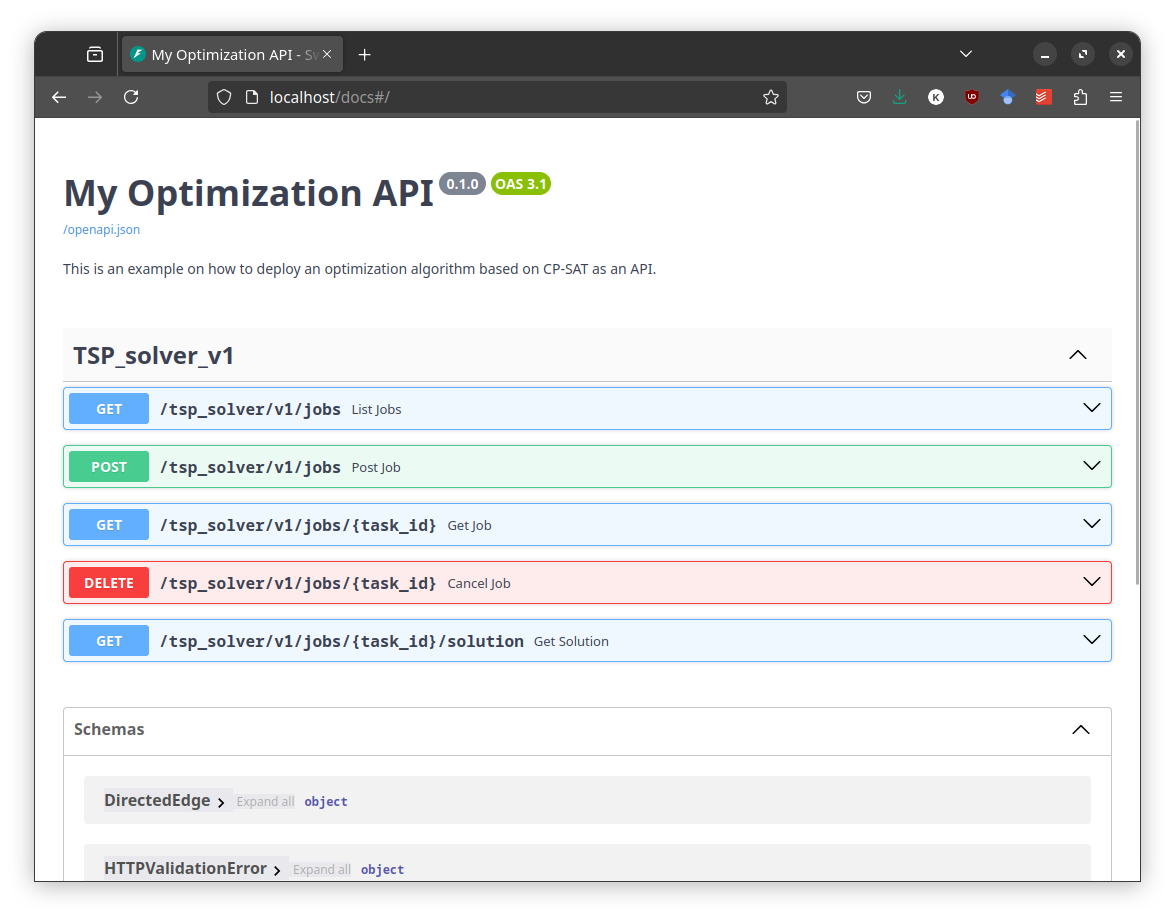 |
|---|
| FastAPI comes with a built-in Swagger UI that allows you to interact with the API. |
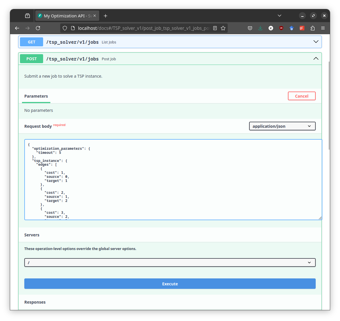 |
|---|
| By clicking on "try it out" you can directly submit a job to the API. |
Here is an instance to try it out
{
  "optimization_parameters": {
    "timeout": 5
  },
  "tsp_instance": {
    "num_nodes": 15,
    "edges": [
      { "source": 0, "target": 1, "cost": 82 },
      { "source": 1, "target": 0, "cost": 82 },
      { "source": 0, "target": 2, "cost": 35 },
      { "source": 2, "target": 0, "cost": 35 },
      { "source": 0, "target": 3, "cost": 58 },
      { "source": 3, "target": 0, "cost": 58 },
      { "source": 0, "target": 4, "cost": 9 },
      { "source": 4, "target": 0, "cost": 9 },
      { "source": 0, "target": 5, "cost": 13 },
      { "source": 5, "target": 0, "cost": 13 },
      { "source": 0, "target": 6, "cost": 91 },
      { "source": 6, "target": 0, "cost": 91 },
      { "source": 0, "target": 7, "cost": 72 },
      { "source": 7, "target": 0, "cost": 72 },
      { "source": 0, "target": 8, "cost": 16 },
      { "source": 8, "target": 0, "cost": 16 },
      { "source": 0, "target": 9, "cost": 50 },
      { "source": 9, "target": 0, "cost": 50 },
      { "source": 0, "target": 10, "cost": 80 },
      { "source": 10, "target": 0, "cost": 80 },
      { "source": 0, "target": 11, "cost": 92 },
      { "source": 11, "target": 0, "cost": 92 },
      { "source": 0, "target": 12, "cost": 28 },
      { "source": 12, "target": 0, "cost": 28 },
      { "source": 0, "target": 13, "cost": 17 },
      { "source": 13, "target": 0, "cost": 17 },
      { "source": 0, "target": 14, "cost": 97 },
      { "source": 14, "target": 0, "cost": 97 },
      { "source": 1, "target": 2, "cost": 14 },
      { "source": 2, "target": 1, "cost": 14 },
      { "source": 1, "target": 3, "cost": 32 },
      { "source": 3, "target": 1, "cost": 32 },
      { "source": 1, "target": 4, "cost": 41 },
      { "source": 4, "target": 1, "cost": 41 },
      { "source": 1, "target": 5, "cost": 52 },
      { "source": 5, "target": 1, "cost": 52 },
      { "source": 1, "target": 6, "cost": 58 },
      { "source": 6, "target": 1, "cost": 58 },
      { "source": 1, "target": 7, "cost": 20 },
      { "source": 7, "target": 1, "cost": 20 },
      { "source": 1, "target": 8, "cost": 1 },
      { "source": 8, "target": 1, "cost": 1 },
      { "source": 1, "target": 9, "cost": 54 },
      { "source": 9, "target": 1, "cost": 54 },
      { "source": 1, "target": 10, "cost": 75 },
      { "source": 10, "target": 1, "cost": 75 },
      { "source": 1, "target": 11, "cost": 15 },
      { "source": 11, "target": 1, "cost": 15 },
      { "source": 1, "target": 12, "cost": 45 },
      { "source": 12, "target": 1, "cost": 45 },
      { "source": 1, "target": 13, "cost": 94 },
      { "source": 13, "target": 1, "cost": 94 },
      { "source": 1, "target": 14, "cost": 41 },
      { "source": 14, "target": 1, "cost": 41 },
      { "source": 2, "target": 3, "cost": 82 },
      { "source": 3, "target": 2, "cost": 82 },
      { "source": 2, "target": 4, "cost": 44 },
      { "source": 4, "target": 2, "cost": 44 },
      { "source": 2, "target": 5, "cost": 83 },
      { "source": 5, "target": 2, "cost": 83 },
      { "source": 2, "target": 6, "cost": 91 },
      { "source": 6, "target": 2, "cost": 91 },
      { "source": 2, "target": 7, "cost": 78 },
      { "source": 7, "target": 2, "cost": 78 },
      { "source": 2, "target": 8, "cost": 51 },
      { "source": 8, "target": 2, "cost": 51 },
      { "source": 2, "target": 9, "cost": 6 },
      { "source": 9, "target": 2, "cost": 6 },
      { "source": 2, "target": 10, "cost": 81 },
      { "source": 10, "target": 2, "cost": 81 },
      { "source": 2, "target": 11, "cost": 77 },
      { "source": 11, "target": 2, "cost": 77 },
      { "source": 2, "target": 12, "cost": 93 },
      { "source": 12, "target": 2, "cost": 93 },
      { "source": 2, "target": 13, "cost": 97 },
      { "source": 13, "target": 2, "cost": 97 },
      { "source": 2, "target": 14, "cost": 33 },
      { "source": 14, "target": 2, "cost": 33 },
      { "source": 3, "target": 4, "cost": 66 },
      { "source": 4, "target": 3, "cost": 66 },
      { "source": 3, "target": 5, "cost": 47 },
      { "source": 5, "target": 3, "cost": 47 },
      { "source": 3, "target": 6, "cost": 54 },
      { "source": 6, "target": 3, "cost": 54 },
      { "source": 3, "target": 7, "cost": 39 },
      { "source": 7, "target": 3, "cost": 39 },
      { "source": 3, "target": 8, "cost": 98 },
      { "source": 8, "target": 3, "cost": 98 },
      { "source": 3, "target": 9, "cost": 90 },
      { "source": 9, "target": 3, "cost": 90 },
      { "source": 3, "target": 10, "cost": 5 },
      { "source": 10, "target": 3, "cost": 5 },
      { "source": 3, "target": 11, "cost": 27 },
      { "source": 11, "target": 3, "cost": 27 },
      { "source": 3, "target": 12, "cost": 61 },
      { "source": 12, "target": 3, "cost": 61 },
      { "source": 3, "target": 13, "cost": 95 },
      { "source": 13, "target": 3, "cost": 95 },
      { "source": 3, "target": 14, "cost": 19 },
      { "source": 14, "target": 3, "cost": 19 },
      { "source": 4, "target": 5, "cost": 34 },
      { "source": 5, "target": 4, "cost": 34 },
      { "source": 4, "target": 6, "cost": 10 },
      { "source": 6, "target": 4, "cost": 10 },
      { "source": 4, "target": 7, "cost": 20 },
      { "source": 7, "target": 4, "cost": 20 },
      { "source": 4, "target": 8, "cost": 44 },
      { "source": 8, "target": 4, "cost": 44 },
      { "source": 4, "target": 9, "cost": 33 },
      { "source": 9, "target": 4, "cost": 33 },
      { "source": 4, "target": 10, "cost": 29 },
      { "source": 10, "target": 4, "cost": 29 },
      { "source": 4, "target": 11, "cost": 36 },
      { "source": 11, "target": 4, "cost": 36 },
      { "source": 4, "target": 12, "cost": 62 },
      { "source": 12, "target": 4, "cost": 62 },
      { "source": 4, "target": 13, "cost": 77 },
      { "source": 13, "target": 4, "cost": 77 },
      { "source": 4, "target": 14, "cost": 63 },
      { "source": 14, "target": 4, "cost": 63 },
      { "source": 5, "target": 6, "cost": 73 },
      { "source": 6, "target": 5, "cost": 73 },
      { "source": 5, "target": 7, "cost": 6 },
      { "source": 7, "target": 5, "cost": 6 },
      { "source": 5, "target": 8, "cost": 91 },
      { "source": 8, "target": 5, "cost": 91 },
      { "source": 5, "target": 9, "cost": 5 },
      { "source": 9, "target": 5, "cost": 5 },
      { "source": 5, "target": 10, "cost": 61 },
      { "source": 10, "target": 5, "cost": 61 },
      { "source": 5, "target": 11, "cost": 11 },
      { "source": 11, "target": 5, "cost": 11 },
      { "source": 5, "target": 12, "cost": 91 },
      { "source": 12, "target": 5, "cost": 91 },
      { "source": 5, "target": 13, "cost": 7 },
      { "source": 13, "target": 5, "cost": 7 },
      { "source": 5, "target": 14, "cost": 88 },
      { "source": 14, "target": 5, "cost": 88 },
      { "source": 6, "target": 7, "cost": 52 },
      { "source": 7, "target": 6, "cost": 52 },
      { "source": 6, "target": 8, "cost": 86 },
      { "source": 8, "target": 6, "cost": 86 },
      { "source": 6, "target": 9, "cost": 48 },
      { "source": 9, "target": 6, "cost": 48 },
      { "source": 6, "target": 10, "cost": 13 },
      { "source": 10, "target": 6, "cost": 13 },
      { "source": 6, "target": 11, "cost": 31 },
      { "source": 11, "target": 6, "cost": 31 },
      { "source": 6, "target": 12, "cost": 91 },
      { "source": 12, "target": 6, "cost": 91 },
      { "source": 6, "target": 13, "cost": 62 },
      { "source": 13, "target": 6, "cost": 62 },
      { "source": 6, "target": 14, "cost": 30 },
      { "source": 14, "target": 6, "cost": 30 },
      { "source": 7, "target": 8, "cost": 79 },
      { "source": 8, "target": 7, "cost": 79 },
      { "source": 7, "target": 9, "cost": 94 },
      { "source": 9, "target": 7, "cost": 94 },
      { "source": 7, "target": 10, "cost": 58 },
      { "source": 10, "target": 7, "cost": 58 },
      { "source": 7, "target": 11, "cost": 12 },
      { "source": 11, "target": 7, "cost": 12 },
      { "source": 7, "target": 12, "cost": 81 },
      { "source": 12, "target": 7, "cost": 81 },
      { "source": 7, "target": 13, "cost": 2 },
      { "source": 13, "target": 7, "cost": 2 },
      { "source": 7, "target": 14, "cost": 89 },
      { "source": 14, "target": 7, "cost": 89 },
      { "source": 8, "target": 9, "cost": 15 },
      { "source": 9, "target": 8, "cost": 15 },
      { "source": 8, "target": 10, "cost": 94 },
      { "source": 10, "target": 8, "cost": 94 },
      { "source": 8, "target": 11, "cost": 23 },
      { "source": 11, "target": 8, "cost": 23 },
      { "source": 8, "target": 12, "cost": 50 },
      { "source": 12, "target": 8, "cost": 50 },
      { "source": 8, "target": 13, "cost": 79 },
      { "source": 13, "target": 8, "cost": 79 },
      { "source": 8, "target": 14, "cost": 65 },
      { "source": 14, "target": 8, "cost": 65 },
      { "source": 9, "target": 10, "cost": 68 },
      { "source": 10, "target": 9, "cost": 68 },
      { "source": 9, "target": 11, "cost": 81 },
      { "source": 11, "target": 9, "cost": 81 },
      { "source": 9, "target": 12, "cost": 34 },
      { "source": 12, "target": 9, "cost": 34 },
      { "source": 9, "target": 13, "cost": 21 },
      { "source": 13, "target": 9, "cost": 21 },
      { "source": 9, "target": 14, "cost": 16 },
      { "source": 14, "target": 9, "cost": 16 },
      { "source": 10, "target": 11, "cost": 10 },
      { "source": 11, "target": 10, "cost": 10 },
      { "source": 10, "target": 12, "cost": 12 },
      { "source": 12, "target": 10, "cost": 12 },
      { "source": 10, "target": 13, "cost": 60 },
      { "source": 13, "target": 10, "cost": 60 },
      { "source": 10, "target": 14, "cost": 61 },
      { "source": 14, "target": 10, "cost": 61 },
      { "source": 11, "target": 12, "cost": 36 },
      { "source": 12, "target": 11, "cost": 36 },
      { "source": 11, "target": 13, "cost": 78 },
      { "source": 13, "target": 11, "cost": 78 },
      { "source": 11, "target": 14, "cost": 79 },
      { "source": 14, "target": 11, "cost": 79 },
      { "source": 12, "target": 13, "cost": 54 },
      { "source": 13, "target": 12, "cost": 54 },
      { "source": 12, "target": 14, "cost": 33 },
      { "source": 14, "target": 12, "cost": 33 },
      { "source": 13, "target": 14, "cost": 29 },
      { "source": 14, "target": 13, "cost": 29 }
    ]
  }
}
Benchmarking your Model
Benchmarking is an essential step if your model is not yet meeting the performance standards of your application or if you are aiming for an academic publication. This process involves analyzing your model's performance, especially important if your model has adjustable parameters. Running your model on a set of predefined instances (a benchmark) allows you to fine-tune these parameters and compare results. Moreover, if alternative models exist, benchmarking helps you ascertain whether your model truly outperforms these competitors.
Designing an effective benchmark is a nuanced task that demands expertise. This section aims to guide you in creating a reliable benchmark suitable for publication purposes.
Given the breadth and complexity of benchmarking, our focus will be on the
basics, particularly through the lens of the Traveling Salesman Problem (TSP),
as previously discussed in the add_circuit section. We refer to the different
model implementations as 'solvers', and we'll explore four specific types:
- A solver employing the
add_circuitapproach. - A solver based on the Miller-Tucker-Zemlin formulation.
- A solver utilizing the Dantzig-Fulkerson-Johnson formulation with iterative addition of subtour constraints until a connected tour is achieved.
- A Gurobi-based solver applying the Dantzig-Fulkerson-Johnson formulation via Lazy Constraints, which are not supported by CP-SAT.
This example highlights common challenges in benchmarking and strategies to address them. A key obstacle in solving NP-hard problems is the variability in solver performance across different instances. For instance, a solver might easily handle a large instance but struggle with a smaller one, and vice versa. Consequently, it's crucial to ensure that your benchmark encompasses a representative variety of instances. This diversity is vital for drawing meaningful conclusions, such as the maximum size of a TSP instance that can be solved or the most effective solver to use.
For a comprehensive exploration of benchmarking, I highly recommend Catherine C. McGeoch's book, "A Guide to Experimental Algorithmics", which offers an in-depth discussion on this topic.
Distinguishing Exploratory and Workhorse Studies in Benchmarking
Before diving into comprehensive benchmarking, it’s essential to conduct preliminary investigations to assess your model’s capabilities and identify any foundational issues. This phase, known as exploratory studies, is crucial for establishing the basis for more detailed benchmarking, subsequently termed as workhorse studies. These latter studies aim to provide reliable answers to specific research questions and are often the core of academic publications. It's important to explicitly differentiate between these two study types and maintain their distinct purposes: exploratory studies for initial understanding and flexibility, and workhorse studies for rigorous, reproducible research.
Exploratory Studies: Foundation Building
Exploratory studies serve as an introduction to both your model and the problem it addresses. This phase is about gaining preliminary understanding and insights.
- Objective: The goal here is to gather early insights rather than definitive conclusions. This phase is instrumental in identifying realistic problem sizes, potential challenges, and narrowing down hyperparameter search spaces.
For instance, in the add_circuit-section, an exploratory study helped us
determine that our focus should be on instances with 100 to 200 nodes. If you
encounter fundamental issues with your model at this stage, it’s advisable to
address these before proceeding to workhorse studies.
Occasionally, the primary performance bottleneck in your model may not be CP-SAT but rather the Python segment where the model is being generated. In these instances, identifying the most resource-intensive parts of your Python code is crucial. I have found the profiler Scalene to be well-suited to investigate and pinpoint these bottlenecks.
Workhorse Studies: Conducting In-depth Evaluations
Workhorse studies follow the exploratory phase, characterized by more structured and meticulous approaches. This stage is vital for a comprehensive evaluation of your model and collecting substantive data for analysis.
- Objective: These studies are designed to answer specific research questions and provide meaningful insights. The approach here is more methodical, focusing on clearly defined research questions. The benchmarks designed should be well-structured and large enough to yield statistically significant results.
Remember, the aim is not to create a flawless benchmark right away but to evolve it as concrete questions emerge and as your understanding of the model and problem deepens. These studies, unlike exploratory ones, will be the focus of your scientific publications, with exploratory studies only referenced for justifying certain design decisions.
Hint: Use the SIGPLAN Empirical Evaluation Checklist if your evaluation has to satisfy academic standards.
Designing a Robust Benchmark for Effective Studies
When undertaking both exploratory and workhorse studies, the creation of a well-designed benchmark is a critical step. This benchmark is the basis upon which you'll test and evaluate your solvers. For exploratory studies, your benchmark can start simple and progressively evolve. However, when it comes to workhorse studies, the design of your benchmark demands meticulous attention to ensure comprehensiveness and reliability.
While exploratory studies also benefit from a thoughtfully designed benchmark—as it accelerates insight acquisition—the primary emphasis at this stage is to have a functioning benchmark in place. This initial benchmark acts as a springboard, providing a foundation for deeper, more detailed analysis in the subsequent workhorse studies. The key is to balance the immediacy of starting with a benchmark against the long-term goal of refining it for more rigorous evaluations.
Ideally, a robust benchmark would consist of a large set of real-world instances, closely reflecting the actual performance of your solver. Real-world instances, however, are often limited in quantity and may not provide enough data for a statistically significant benchmark. In such cases, it's advisable to explore existing benchmarks from literature, like the TSPLIB for TSP. Leveraging established benchmarks allows for comparison with prior studies, but be cautious about their quality, as not all are equally well-constructed. For example, TSPLIB's limitations in terms of instance size variation and heterogeneity can hinder result aggregation.
Therefore, creating custom instances might be necessary. When doing so, aim for enough instances per size category to establish reliable and statistically significant data points. For instance, generating 10 instances for each size category (e.g., 25, 50, 75, 100, 150, 200, 250, 300, 350, 400, 450, 500) can provide a solid basis for analysis. This approach, though modest in scale, suffices to illustrate the benchmarking process.
Exercise caution with random instance generators, as they may not accurately represent real-world scenarios. For example, randomly generated TSP instances might lack collinear points common in real-world situations, like houses aligned on straight roads, or they might not replicate real-world clustering patterns. To better mimic reality, incorporate real-world data or use diverse generation methods to ensure a broader variety of instances. For the TSP, we could for example also have sampled from the larger TSPLIB instances.
Consider conducting your evaluation using two distinct benchmarks, especially when dealing with different data types. For instance, you might have one benchmark derived from real-world data which, although highly relevant, is too limited in size to provide robust statistical insights. Simultaneously, you could use a second benchmark based on a larger set of random instances, better suited for detailed statistical analysis. This dual-benchmark approach allows you to demonstrate the consistency and reliability of your results, ensuring they are not merely artifacts of a particular dataset's characteristics. It's a strategy that adds depth to your evaluation, showcasing the robustness of your findings across varied data sources. We will use this approach below, generating robust plots from random instances, but also comparing them to real-world instances. Mixing the two benchmarks would not be advisable, as the random instances would dominate the results.
Lastly, always separate the creation of your benchmark from the execution of experiments. Create and save instances in a separate process to minimize errors. The goal is to make your evaluation as error-proof as possible, avoiding the frustration and wasted effort of basing decisions on flawed data. Be particularly cautious with pseudo-random number generators; while theoretically deterministic, their use can inadvertently lead to irreproducible results. Sharing benchmarks is also more straightforward when you can distribute the instances themselves, rather than the code used to generate them.
Efficiently Managing Your Benchmarks
Managing benchmark data can become complex, especially with multiple experiments and research questions. Here are some strategies to keep things organized:
- Folder Structure: Maintain a clear folder structure for your experiments,
with a top-level
evaluationsfolder and descriptive subfolders for each experiment. For our experiment we have the following structure:evaluations ├── tsp │ ├── 2023-11-18_random_euclidean │ │ ├── PRIVATE_DATA │ │ │ ├── ... all data for debugging │ │ ├── PUBLIC_DATA │ │ │ ├── ... selected data to share │ │ ├── README.md: Provide a short description of the experiment │ │ ├── 00_generate_instances.py │ │ ├── 01_run_experiments.py │ │ ├── .... │ ├── 2023-11-18_tsplib │ │ ├── PRIVATE_DATA │ │ │ ├── ... all data for debugging │ │ ├── PUBLIC_DATA │ │ │ ├── ... selected data to share │ │ ├── README.md: Provide a short description of the experiment │ │ ├── 01_run_experiments.py │ │ ├── .... - Redundancy and Documentation: While some redundancy is acceptable, comprehensive documentation of each experiment is crucial for future reference.
- Simplified Results: Keep a streamlined version of your results for easy access, especially for plotting and sharing.
- Data Storage: Save all your data, even if it seems insignificant at the time. This ensures you have a comprehensive dataset for later analysis or unexpected inquiries. Because this can become a lot of data, it's advisable to have two folders: One with all data and one with a selection of data that you want to share.
- Experiment Flexibility: Design experiments to be interruptible and extendable, allowing for easy resumption or modification. This is especially important for exploratory studies, where you may need to make frequent adjustments. However, if your workhorse study takes a long time to run, you do not want to repeat it from scratch if you want to add a further solver.
- Utilizing Technology: Employ tools like slurm for efficient distribution of experiments across computing clusters, saving time and resources. The faster you have your results, the faster you can act on them.
Due to a lack of tools that exactly fitted my needs I developed AlgBench to manage the results, and Slurminade to easily distribute the experiments on a cluster via a simple decorator. However, there may be better tools out there, now, especially from the Machine Learning community. Drop me a quick mail if you have found some tools you are happy with, and I will take a look myself.
Analyzing the results
Let us now come to the actual analysis of the results. We will focus on the following questions:
- Up to which size can we solve TSP instances with the different solvers?
- Which solver is the fastest?
- How does the performance change if we increase the optimality tolerance?
Our Benchmarks: We executed the four solvers with a time limit of 90s and the optimality tolerances [0.1%, 1%, 5%, 10%, 25%] on a random benchmark set and a TSPLIB benchmark set. The random benchmark set consists of 10 instances for each number of nodes
[25, 50, 75, 100, 150, 200, 250, 300, 350, 400, 450, 500]. The weights were chosen based on randomly embedding the nodes into a 2D plane and using the Euclidean distances. The TSPLIB benchmark consists of all Euclidean instances with less than 500 nodes. It is critical to have a time limit, as otherwise, the benchmarks would take forever. You can find all find the whole experiment here.
Let us first look at the results of the random benchmark, as they are easier to interpret. We will then compare them to the TSPLIB benchmark.
Random Instances
A common, yet simplistic method to assess a model's performance involves plotting its runtime against the size of the instances it processes. However, this approach can often lead to inaccurate interpretations, particularly because time-limited cutoffs can disproportionately affect the results. Instead of the expected exponential curves, you will get skewed sigmoidal curves. Consequently, such plots might not provide a clear understanding of the instance sizes your model is capable of handling efficiently.
 |
|---|
| The runtimes are sigmoidal instead of exponential because the time limit skews the results. The runtime can frequently exceed the time limit, because of expensive model building, etc. Thus, a pure runtime plot says surprisingly little (or is misleading) and can usually be discarded. |
To gain a more accurate insight into the capacities of your model, consider plotting the proportion of instances of a certain size that your model successfully solves. This method requires a well-structured benchmark to yield meaningful statistics for each data point. Without this structure, the resulting curve may appear erratic, making it challenging to draw dependable conclusions.
 |
|---|
| For each x-value: What are the chances (y-values) that a model of this size (x) can be solved? |
Furthermore, if the pursuit is not limited to optimal solutions but extends to encompass solutions of acceptable quality, the analysis can be expanded. One can plot the number of instances that the model solves within a defined optimality tolerance, as demonstrated in the subsequent figure:
 |
|---|
| For each x-value: What are the chances (y-values) that a model of this size (x) can be solved to what quality (line style)? |
For a comparative analysis across various models against an arbitrary benchmark, cactus plots emerge as a potent tool. These plots illustrate the number of instances solved over time, providing a clear depiction of a model's efficiency. For example, a coordinate of $x=10, y=20$ on such a plot signifies that 20 instances were solved within a span of 10 seconds each. It is important to note, however, that these plots do not facilitate predictions for any specific instance unless the benchmark set is thoroughly familiar. They do allow for an estimation of which model is quicker for simpler instances and which can handle more challenging instances within a reasonable timeframe. The question of what exactly is a simple or challenging instance, however, is better answered by the previous plots.
Cactus plots are notably prevalent in the evaluation of SAT-solvers, where instance size is a poor indicator of difficulty. A more detailed discussion on this subject can be found in the referenced academic paper: Benchmarking Solvers, SAT-style by Brain, Davenport, and Griggio
 |
|---|
| For each x-value: How many (y) of the benchmark instances could have been solved with this time limit (x)? |
Additionally, the analysis can be refined to account for different quality tolerances. This requires either multiple experimental runs or tracking the progression of the lower and upper bounds within the solver. In the context of CP-SAT, for instance, this tracking can be implemented via the Solution Callback, although its activation is may depend on updates to the objective rather than the bounds.
 |
|---|
| For each x-value: How many (y) of the benchmark instances could have been solved to a specific quality (line style) with this time limit (x)? |
Instead of plotting the number of solved instances, one can also plot the number of unsolved instances over time. This can be easier to read and additionally indicates the number of instances in the benchmark. However, I personally do not have a preference for one or the other, and would recommend using the one that is more intuitive to read for you.
TSPLIB
Our second benchmark for the Traveling Salesman Problem leverages the TSPLIB, a set of instances based on real-world data. This will introduce two challenges:
- The difficulty in aggregating benchmark data due to its limited size and heterogeneous nature.
- Notable disparities in results, arising from the differing characteristics of random and real-world instances.
The irregularity in instance sizes makes traditional plotting methods, like plotting the number of solved instances over time, less effective. While data smoothing methods, such as rolling averages, are available, they too have their limitations.
 |
|---|
| Such a plot may prove inefficient when dealing with high variability, particularly when some data points are underrepresented. |
In contrast, the cactus plot still provides a clear and comprehensive
perspective of various model performances. An interesting observation we can
clearly see in it, is the diminished capability of the "Iterative Dantzig" model
in solving instances, and a closer performance alignment between the
add_circuit and Gurobi models.
 |
|---|
| Cactus plots maintain clarity and relevance, and show a performance differences between TSPLib and random instances. |
However, since cactus plots do not offer insights into individual instances,
it's beneficial to complement them with a detailed table of results for the
specific model you are focusing on. This approach ensures a more nuanced
understanding of model performance across varied instances. The following table
provides the results for the add_circuit-model.
| Instance | # nodes | runtime | lower bound | objective | opt. gap |
|---|---|---|---|---|---|
| att48 | 48 | 0.47 | 33522 | 33522 | 0 |
| eil51 | 51 | 0.69 | 426 | 426 | 0 |
| st70 | 70 | 0.8 | 675 | 675 | 0 |
| eil76 | 76 | 2.49 | 538 | 538 | 0 |
| pr76 | 76 | 54.36 | 108159 | 108159 | 0 |
| kroD100 | 100 | 9.72 | 21294 | 21294 | 0 |
| kroC100 | 100 | 5.57 | 20749 | 20749 | 0 |
| kroB100 | 100 | 6.2 | 22141 | 22141 | 0 |
| kroE100 | 100 | 9.06 | 22049 | 22068 | 0 |
| kroA100 | 100 | 8.41 | 21282 | 21282 | 0 |
| eil101 | 101 | 2.24 | 629 | 629 | 0 |
| lin105 | 105 | 1.37 | 14379 | 14379 | 0 |
| pr107 | 107 | 1.2 | 44303 | 44303 | 0 |
| pr124 | 124 | 33.8 | 59009 | 59030 | 0 |
| pr136 | 136 | 35.98 | 96767 | 96861 | 0 |
| pr144 | 144 | 21.27 | 58534 | 58571 | 0 |
| kroB150 | 150 | 58.44 | 26130 | 26130 | 0 |
| kroA150 | 150 | 90.94 | 26498 | 26977 | 2% |
| pr152 | 152 | 15.28 | 73682 | 73682 | 0 |
| kroA200 | 200 | 90.99 | 29209 | 29459 | 1% |
| kroB200 | 200 | 31.69 | 29437 | 29437 | 0 |
| pr226 | 226 | 74.61 | 80369 | 80369 | 0 |
| gil262 | 262 | 91.58 | 2365 | 2416 | 2% |
| pr264 | 264 | 92.03 | 49121 | 49512 | 1% |
| pr299 | 299 | 92.18 | 47709 | 49217 | 3% |
| linhp318 | 318 | 92.45 | 41915 | 52032 | 19% |
| lin318 | 318 | 92.43 | 41915 | 52025 | 19% |
| pr439 | 439 | 94.22 | 105610 | 163452 | 35% |
A last option is to split the y-axis into the part where the solving time is still within the time limit, and the part where it is not and the optimality gap becomes relevant. Such a plot has some benefits but can also be difficult to scale or aggregate.
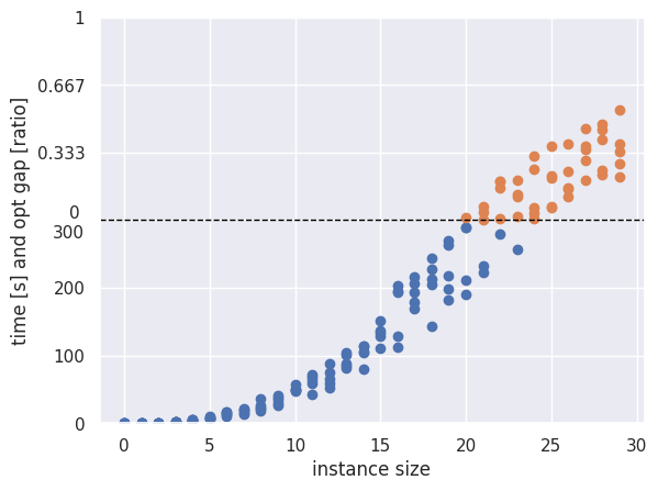 |
|---|
| This plot splits the y-axis into a part where the instances can still be solved within the time limit, such that the time can be shown, and the part where the time limit is exceeded, such that the optimality gap can be shown. This example was generated by my student assistant Rouven Kniep, and he is working on creating an easy-to-use script for such plots. |
This should highlight that often you need a combination of different benchmarks and plots to get a good understanding of the performance of your model.
Conclusion
Benchmarking solvers for NP-hard problems is not as straightforward as it might seem at first. There are many pitfalls and often there is no perfect solution. On the example of the TSP, we have seen how we can still get some useful results and nice plots on which we can base our decisions.
If you want to make an automated decision on what model/solver to use, things can get complicated. Often, there is none that dominates on all instances. If you want a single metric for comparing the performance, there is no perfect solution. I am actually the technical lead and co-organizer of a yearly challenge on solving hard optimization problems in computational geometry CG:SHOP, which is part of CG Week. Here, I am confronted with scoring the solutions of the participants, without having any useful bounds. It turned out that giving a score between zero and one for each instance, based on the squared difference to the best solution, works quite well. While it still has flaws, it is showed to be relatively fair and robust. The general problem of selecting the right strategy for a specific instance is called Algorithm Selection problem and can be surprisingly complex, too.
Using CP-SAT for Bigger Problems with Large Neighborhood Search
CP-SAT is great at solving small and medium-sized problems. But what if you have a really big problem on your hands? One option might be to use a special kind of algorithm known as a "meta-heuristic", like a genetic algorithm. But these can be hard to set up and might not even give you good results.
Sometimes you will see new algorithms with cool-sounding names in scientific papers. While tempting, these are often just small twists on older methods and might leave out key details that make them work. If you are interested, there's a discussion about this issue in a paper by Sörensen, called "Metaheuristics – The Metaphor Exposed".
The good news? You do not have to implement an algorithm that simulates the mating behavior of forest frogs to solve your problem. If you already know how to use CP-SAT, you can stick with it to solve big problems without adding unnecessary complications. Even better? This technique, called Large Neighborhood Search, often outperforms all other approaches.
What Sets Large Neighborhood Search Apart?
Many traditional methods generate several "neighbor" options around an existing solution and pick the best one. However, making each neighbor solution takes time, limiting how many you can examine.
Large Neighborhood Search (LNS) offers a more efficient approach. Instead of generating neighbors one by one, LNS formulates a "mini-problem" that modifies parts of the current solution. This often involves randomly selecting some variables, resetting them, and using CP-SAT (or a similar tool) to find the optimal new values within the context of the remaining solution. This method, known as "destroy and repair," allows for a broader exploration of neighbor solutions without constructing each one individually.
Moreover, LNS can easily be mixed with other methods like genetic algorithms. If you are already using a genetic algorithm, you could supercharge it by applying CP-SAT to find the best possible crossover of two or more existing solutions. It is like genetic engineering, but without any ethical worries!
When looking into the logs of CP-SAT, you may notice that it uses LNS itself to find better solutions.
8 incomplete subsolvers: [feasibility_pump, graph_arc_lns, graph_cst_lns, graph_dec_lns, graph_var_lns, rins/rens, rnd_cst_lns, rnd_var_lns]Why does it not suffice to just run CP-SAT if it already solves the problem with LNS? The reason is that CP-SAT has to be relatively problem-agnostic. It has no way of knowing the structure of your problem and thus cannot use this information to improve the search. You on the other hand know a lot about your problem and can use this knowledge to implement a more efficient version.
Literature:
- General Paper on LNS-variants: Pisinger and Ropke - 2010
- A generic variant (RINS), that is also used by CP-SAT: Danna et al. 2005
We will now look into some examples to see this approach in action.
Example 1: Knapsack
You are given a knapsack that can carry a certain weight limit $C$, and you have various items $I$ you can put into it. Each item $i\in I$ has a weight $w_i$ and a value $v_i$. The goal is to pick items to maximize the total value while staying within the weight limit.
\max \sum_{i \in I} v_i x_i\text{s.t.} \sum_{i \in I} w_i x_i \leq Cx_i \in \\{0,1\\}This is one of the simplest NP-hard problems and can be solved with a dynamic programming approach in pseudo-polynomial time. CP-SAT is also able to solve many large instances of this problem in an instant. However, its simple structure makes it a good example to demonstrate the use of Large Neighborhood Search, even if the algorithm will not be of much use for this problem.
A simple idea for the LNS is to delete some elements from the current solution, compute the remaining capacity after deletion, select some additional items from the remaining items, and try to find the optimal solution to fill the remaining capacity with the deleted items and the newly selected items. Repeat this until you are happy with the solution quality. The number of items you delete and select can be fixed such that the problem can be easily solved by CP-SAT. You can find a full implementation under examples/lns_knapsack.ipynb.
Let us look only on an example here:
Instance: $C=151$, $I=I{0}(w=12, v=37),I{1}(w=16, v=49),I{2}(w=20, v=53),I{3}(w=11, v=14),I{4}(w=19, v=42),$ $\quad I{5}(w=13, v=53),I{6}(w=18, v=54),I{7}(w=16, v=56),I{8}(w=14, v=45),I{9}(w=12, v=39),$ $\quad I{10}(w=11, v=42),I{11}(w=19, v=43),I{12}(w=12, v=43),I{13}(w=19, v=66),I{14}(w=20, v=54),$ $\quad I{15}(w=13, v=54),I{16}(w=12, v=33),I{17}(w=12, v=38),I{18}(w=14, v=43),I{19}(w=15, v=28),$ $\quad I{20}(w=11, v=47),I{21}(w=10, v=31),I{22}(w=20, v=97),I{23}(w=10, v=35),I{24}(w=19, v=56),$ $\quad I{25}(w=11, v=33),I{26}(w=12, v=38),I{27}(w=15, v=45),I{28}(w=17, v=58),I{29}(w=11, v=48),$ $\quad I{30}(w=15, v=32),I{31}(w=17, v=67),I{32}(w=15, v=43),I{33}(w=16, v=41),I{34}(w=18, v=42),$ $\quad I{35}(w=14, v=44),I{36}(w=20, v=45),I{37}(w=13, v=50),I{38}(w=17, v=57),I{39}(w=17, v=33),$ $\quad I{40}(w=17, v=49),I{41}(w=12, v=21),I{42}(w=14, v=37),I{43}(w=20, v=74),I{44}(w=14, v=55),$ $\quad I{45}(w=10, v=25),I{46}(w=16, v=26),I{47}(w=10, v=37),I{48}(w=18, v=63),I{49}(w=16, v=39),$ $\quad I{50}(w=16, v=57),I{51}(w=16, v=47),I{52}(w=10, v=43),I{53}(w=12, v=30),I{54}(w=12, v=40),$ $\quad I{55}(w=19, v=48),I{56}(w=12, v=39),I{57}(w=14, v=43),I{58}(w=17, v=35),I{59}(w=19, v=51),$ $\quad I{60}(w=16, v=48),I{61}(w=19, v=72),I{62}(w=16, v=45),I{63}(w=19, v=88),I{64}(w=15, v=20),$ $\quad I{65}(w=17, v=49),I{66}(w=14, v=40),I{67}(w=14, v=27),I{68}(w=19, v=51),I{69}(w=10, v=37),$ $\quad I{70}(w=15, v=42),I{71}(w=13, v=29),I{72}(w=20, v=87),I{73}(w=13, v=28),I{74}(w=15, v=38),$ $\quad I{75}(w=19, v=77),I{76}(w=13, v=35),I{77}(w=17, v=55),I{78}(w=13, v=39),I{79}(w=10, v=26),$ $\quad I{80}(w=15, v=32),I{81}(w=12, v=40),I{82}(w=11, v=21),I{83}(w=18, v=82),I{84}(w=13, v=41),$ $\quad I{85}(w=12, v=27),I{86}(w=15, v=35),I{87}(w=18, v=48),I{88}(w=15, v=64),I{89}(w=19, v=62),$ $\quad I{90}(w=20, v=64),I{91}(w=13, v=45),I{92}(w=19, v=64),I{93}(w=18, v=83),I{94}(w=11, v=38),$ $\quad I{95}(w=10, v=30),I{96}(w=18, v=65),I{97}(w=19, v=56),I{98}(w=12, v=41),I{99}(w=17, v=36)$
Initial solution of value 442: $\{I{0}, I{1}, I{2}, I{3}, I{4}, I{5}, I{6}, I{7}, I{8}, I{9}\}$
We will now repeatedly delete 5 items from the current solution and try to fill the newly gained capacity with an optimal solution built from the deleted items and 10 additional items. Note that this approach essentially considers $2^{5+10}=32768$ neighbored solutions in each iteration. However, we could easily scale it up to consider $2^{100+900}\sim 10^{300}$ neighbored solutions in each iteration thanks to the implicit representation of the neighbored solutions and CP-SAT ability to prune large parts of the search space.
Round 1 of LNS algorithm:
- Deleting the following 5 items from the solution: $\{I{0}, I{7}, I{8}, I{9}, I_{6}\}$
- Repairing solution by considering the following subproblem:
- Subproblem: $C=72$, $I=\{I{6},I{9},I{86},I{13},I{47},I{73},I{0},I{8},I{7},I{38},I{57},I{11},I{60},I{14}\}$
- Computed the following solution of value 244 for the subproblem: $\{I{8}, I{9}, I{13}, I{38}, I_{47}\}$
- Combining $\{I{1}, I{2}, I{3}, I{4}, I{5}\}\cup \{I{8}, I{9}, I{13}, I{38}, I{47}\}$
- New solution of value 455: $\{I{1}, I{2}, I{3}, I{4}, I{5}, I{8}, I{9}, I{13}, I{38}, I{47}\}$
Round 2 of LNS algorithm:
- Deleting the following 5 items from the solution: $\{I{3}, I{13}, I{2}, I{9}, I_{1}\}$
- Repairing solution by considering the following subproblem:
- Subproblem: $C=78$, $I=\{I{13},I{9},I{84},I{41},I{15},I{42},I{74},I{16},I{3},I{1},I{2},I{67},I{50},I{89},I_{43}\}$
- Computed the following solution of value 275 for the subproblem: $\{I{1}, I{15}, I{43}, I{50}, I_{84}\}$
- Combining $\{I{4}, I{5}, I{8}, I{38}, I{47}\}\cup \{I{1}, I{15}, I{43}, I{50}, I{84}\}$
- New solution of value 509: $\{I{1}, I{4}, I{5}, I{8}, I{15}, I{38}, I{43}, I{47}, I{50}, I{84}\}$
Round 3 of LNS algorithm:
- Deleting the following 5 items from the solution: $\{I{8}, I{43}, I{84}, I{1}, I_{50}\}$
- Repairing solution by considering the following subproblem:
- Subproblem: $C=79$, $I=\{I{84},I{76},I{34},I{16},I{37},I{20},I{8},I{43},I{50},I{1},I{12},I{35},I_{53}\}$
- Computed the following solution of value 283 for the subproblem: $\{I{8}, I{12}, I{20}, I{37}, I{50}, I{84}\}$
- Combining $\{I{4}, I{5}, I{15}, I{38}, I{47}\}\cup \{I{8}, I{12}, I{20}, I{37}, I{50}, I_{84}\}$
- New solution of value 526: $\{I{4}, I{5}, I{8}, I{12}, I{15}, I{20}, I{37}, I{38}, I{47}, I{50}, I_{84}\}$
Round 4 of LNS algorithm:
- Deleting the following 5 items from the solution: $\{I{37}, I{4}, I{20}, I{5}, I_{15}\}$
- Repairing solution by considering the following subproblem:
- Subproblem: $C=69$, $I=\{I{37},I{4},I{20},I{15},I{82},I{41},I{56},I{76},I{85},I{5},I{32},I{57},I{7},I{67}\}$
- Computed the following solution of value 260 for the subproblem: $\{I{5}, I{7}, I{15}, I{20}, I_{37}\}$
- Combining $\{I{8}, I{12}, I{38}, I{47}, I{50}, I{84}\}\cup \{I{5}, I{7}, I{15}, I{20}, I_{37}\}$
- New solution of value 540: $\{I{5}, I{7}, I{8}, I{12}, I{15}, I{20}, I{37}, I{38}, I{47}, I{50}, I_{84}\}$
Round 5 of LNS algorithm:
- Deleting the following 5 items from the solution: $\{I{38}, I{12}, I{20}, I{47}, I_{37}\}$
- Repairing solution by considering the following subproblem:
- Subproblem: $C=66$, $I=\{I{20},I{47},I{37},I{86},I{58},I{56},I{54},I{38},I{12},I{39},I{68},I{75},I{66},I{2},I_{99}\}$
- Computed the following solution of value 254 for the subproblem: $\{I{12}, I{20}, I{37}, I{47}, I_{75}\}$
- Combining $\{I{5}, I{7}, I{8}, I{15}, I{50}, I{84}\}\cup \{I{12}, I{20}, I{37}, I{47}, I_{75}\}$
- New solution of value 560: $\{I{5}, I{7}, I{8}, I{12}, I{15}, I{20}, I{37}, I{47}, I{50}, I{75}, I_{84}\}$
Example 2: Different Neighborhoods for the Traveling Salesman Problem
Simply removing a portion of the solution and then trying to fix it is not the most effective approach. In this section, we will explore various neighborhoods for the Traveling Salesman Problem (TSP). The geometry of TSP not only permits advantageous neighborhoods but also offers visually appealing representations. When you have several neighborhood strategies, they can be dynamically integrated using an Adaptive Large Neighborhood Search (ALNS).
The image illustrates an optimization process for a tour that needs to traverse the green areas, factoring in turn costs, within an embedded graph (mesh). The optimization involves choosing specific regions (highlighted in red) and calculating the optimal tour within them. As iterations progress, the initial tour generally improves, although some iterations may not yield any enhancement. Regions in red are selected due to the high cost of the tour within them. Once optimized, the center of that region is added to a tabu list, preventing it from being chosen again.
 |
|---|
| Large Neighbordhood Search for Coverage Path Planning by repeatedly selecting a geometric region (red) and optimizing the tour within it. The red parts of the tour highlight the changes in the iteration. Read from left to right, and from up to down. |
How can you determine the appropriate size of a region to select? You have two main options: conduct preliminary experiments or adjust the size adaptively during the search. Simply allocate a time limit for each iteration. If the solver does not optimize within that timeframe, decrease the region size. Conversely, if it does, increase the size. Utilizing exponential factors will help the size swiftly converge to its optimal dimension. However, it's essential to note that this method assumes subproblems are of comparable difficulty and may necessitate additional conditions.
For the Euclidean TSP, as opposed to a mesh, optimizing regions is not straightforward. Multiple effective strategies exist, such as employing a segment from the previous tour rather than a geometric region. By implementing various neighborhoods and evaluating their success rates, you can allocate a higher selection probability to the top-performing ones. This approach is demonstrated in an animation crafted by two of my students, Gabriel Gehrke and Laurenz Illner. They incorporated four distinct neighborhoods and utilized ALNS to dynamically select the most effective one.
 |
|---|
| Animation of an Adaptive Large Neighborhood Search for the classical Traveling Salesman Problem. It uses four different neighborhood strategies which are selected randomly with a probability based on their success rate in previous iterations. If you check the logs of the latest (v9.8) version of CP-SAT, it also rates the performance of its LNS-strategies and uses the best performing strategies more often (UCB1-algorithm). |
Multi-Armed Bandit: Exploration vs. Exploitation
Having multiple strategies for each iteration of your LNS available is great, but how do you decide which one to use? You could just pick one randomly, but this is not very efficient as it is unlikely to select the best one. You could also use the strategy that worked best in the past, but maybe there is a better one you have not tried yet. This is the so-called exploration vs. exploitation dilemma. You want to exploit the strategies that worked well in the past, but you also want to explore new strategies to find even better ones. Luckily, this problem has been studied extensively as the Multi-Armed Bandit Problem for decades, and there are many good solutions. One of the most popular ones is the Upper Confidence Bound (UCB1) algorithm, which is also used by CP-SAT. In the following, you can see the a LNS-statistic of the CP-SATs strategies.
LNS stats                Improv/Calls  Closed  Difficulty  TimeLimit
       'graph_arc_lns':          5/65     49%        0.26       0.10
       'graph_cst_lns':          4/65     54%        0.47       0.10
       'graph_dec_lns':          3/65     49%        0.26       0.10
       'graph_var_lns':          4/66     55%        0.56       0.10
           'rins/rens':         23/66     39%        0.03       0.10
         'rnd_cst_lns':         12/66     50%        0.19       0.10
         'rnd_var_lns':          6/66     52%        0.36       0.10
    'routing_path_lns':         41/65     48%        0.10       0.10
  'routing_random_lns':         24/65     52%        0.26       0.10
We will not dig into the details of the algorithm here, but if you are interested, you can find many good resources online. I just wanted to make you aware of the exploration vs. exploitation dilemma and that many smart people have already thought about it.
TODO: Continue...