ChromaR Documentation

ChromaR is an experimental R toolkit for analyzing and exploring chromatic storytelling in movies or any other video source. What does this actually mean? You can check it reading this two articles:

• Getting StartedExploring chromatic storytelling in movies with R: Introduction
• Exploring chromatic storytelling in movies with R: the ChromaR package

This documentation assumes that the reader is already familiar with R. If not so, a gentle introduction to R can be found here.

_{Examples of framelines}

Summary

• Getting Started
• Additional Features
• Generate your own dataset
• Built With
• Authors
• Acknowledgements
• License

Getting Started

Installing ChromaR

The ChromaR package is hosted on GitHub and must be therefore installed through Devtools:

> install.packages("devtools")
> library(devtools)
> install_github("detsutut/chroma", subdir="chromaR")
> library(chromaR)

Inspecting Default Datasets

ChromaR exposes two ready-to-go databases you can use for practice purposes: Matrix and Miyazaki. These two lists collect the movie datasets for the Matrix trilogy and Miyazaki's (partial) filmography. Let's look at the latter, focusing then on "Princess Mononoke":

> miyazaki = chromaR::miyazaki
> miyazaki_grouped = lapply(miyazaki, function(movie){groupframes(movie,seconds=5)})
> getSummary(miyazaki_grouped)

           R         G        B       lum duration     RGB                                     title frameId
1   95.43707  84.02420 76.22149  86.58976     7020 #5F544C 1984 - Nausicaa of the Valley of the Wind       1
2   70.16424  72.72785 70.92556  71.76052     7470 #464846           1986 - Laputa Castle in the Sky       2
3   75.58941  82.22896 74.08047  79.34076     5185 #4B524A                 1988 - My Neighbor Totoro       3
4   85.45816  93.22114 88.66284  90.39083     5595 #555D58                        1992 - Porco Rosso       4
5   58.40236  65.24263 61.49390  62.77819     7995 #3A413D                  1997 - Princess Mononoke       5
6   77.02667  87.91691 91.37884  85.03065     6180 #4D575B            1998 - Kiki's Delivery Service       6
7   95.17101  83.02897 68.00188  85.01860     7470 #5F5344                     2001  - Spirited Away       7
8   81.94425  77.87252 67.05723  77.90436     7145 #514D43               2005 - Howl's Moving Castle       8
9  105.48353 112.59336 96.48504 108.68850     6045 #697060      2008 - Ponyo on the Cliff by the Sea       9
10  92.98617  97.15226 80.36500  94.05584     7585 #5C6150                     2013 - The Wind Rises      10

First, we applied the groupframesfunction to each movie in the collection, then we displayed a summary of it through getSummary, which shows the average RGB triplet for each movie along with other details. Moving to the single movie, let's look into Princess Mononoke:

> mononoke = miyazaki[[5]]
> attr(mononoke, "title")

"1997 - Princess Mononoke"

> mononoke[sample(nrow(mononoke),5),]

frameId R       G       B       hex     lum      
99055   112.930 125.730 95.100  #707D5F 118.52070
157672  62.832  54.164  57.341  #3E3639 57.11387 
80875   66.538  77.007  84.124  #424D54 74.64917  
19967   56.969  106.630 111.510 #386A6F 92.26850 
159740  44.664  49.680  60.627  #2C313C 49.37937

Here we see 5 random rows from the Mononoke dataset. Each row represents a single frame of the movie. For each frame, we collect the average R, G and B value, its Hex string equivalent and the average luminance. This is all we need to plot the framelines.

Plotting the First Frameline

In order to draw a nice plot for Mononoke, we have to merge the frames together first.

> mononoke_grouped = groupframes(mononoke, seconds = 10)
> plotFrameline(mononoke_grouped, verbose = 1)

_Mononoke

Here we use a 10 seconds merging window, but you can try to set bigger values to get thicker bars. If the seconds argument is not provided, a merging time window will be calculated automatically.

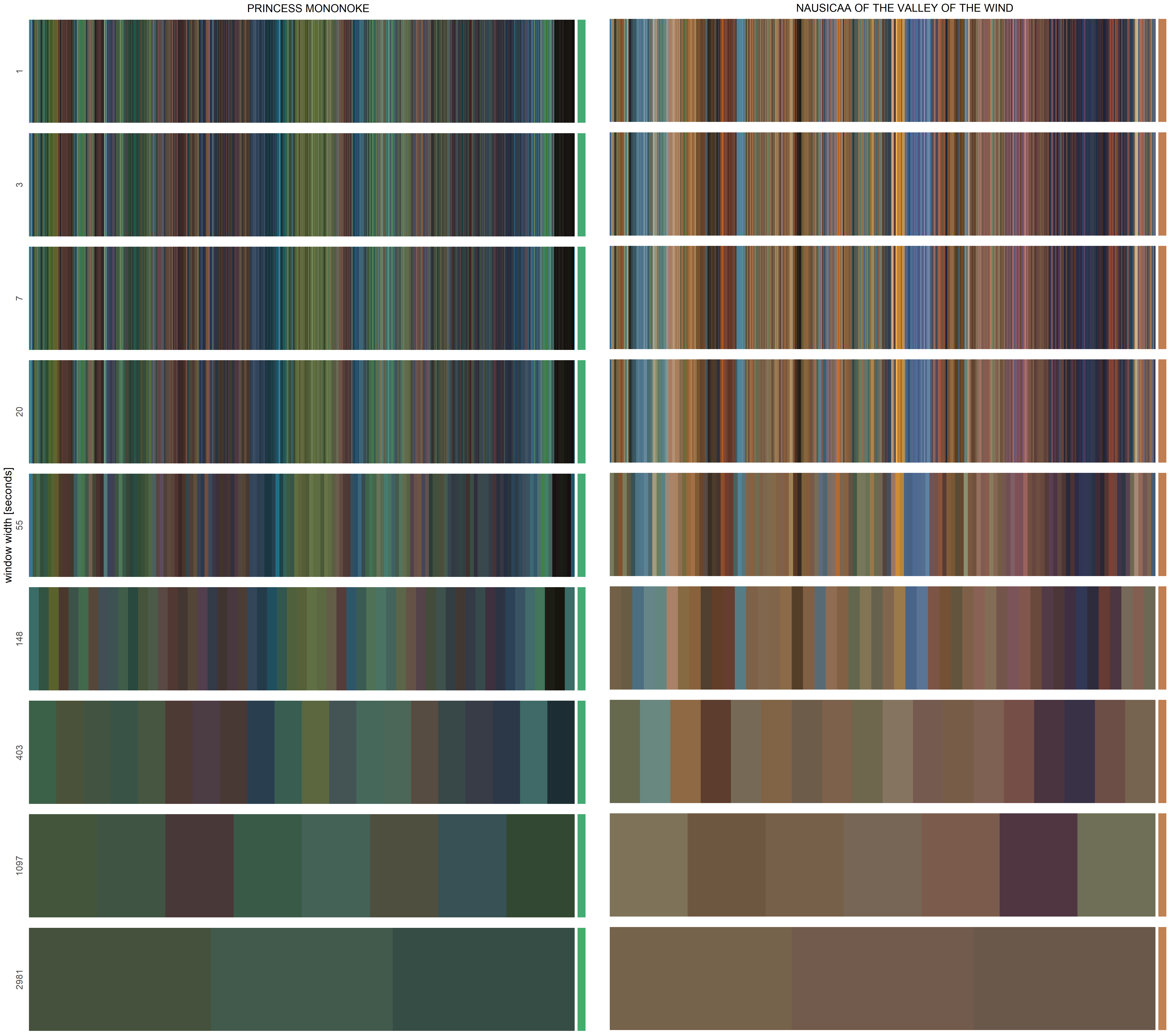
_{Changing the merging window width changes the appearance of the plot}

Additional Features

Time Windows

When we merge frames together through groupframes, the time window we pick with the seconds argument will affect the aesthetic outcome of our plot. In fact, depending on this parameter, the resulting frameline could be sharp or very blurred. A 5-seconds window is usually fine for most of the movies, but you can visually tune it using the 'plotTimeWindows' function.

> nausicaa = chromaR::miyazaki[[1]]
> plotTimeWindows(nausicaa)

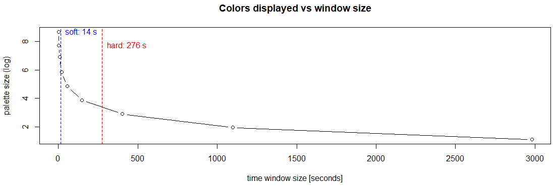
_{The algorithm suggests two different cutoffs: a soft one (sharp frameline, most of the color information is preserved) and a hard one (blurried frameline, defined by the time constant of the exponential decay)}

_{…or you can simply pick up your favourite window size by visual inspection}

Summary Tiles

A chromatic study on entire seasons or movie franchises can be focused on many different features. Summaries about luminance, hue and saturation can be retrieved using the getSummary function.

> ldr = getFrames()
> ldr.grouped = lapply(ldr,function(x){groupframes(x,seconds = 5)})
> ldr.summary = getSummary(ldr.grouped)

> plotTilesSummary(ldr.summary,
                 mode = "lum",                      #lum = luminance, h = hue, s = saturation
                 verbose = 1,
                 title = "Love Death & Robots",
                 subtitle = "Brightness")

_{Netflix's Love, Death & Robots brightness summary}

_{Netflix's Love, Death & Robots summary for hue and saturation}

Channels Temporal Inspection

ChromaR exposes some useful function to inspect color channels' trends over time. The temperature function measures and plot the distance of the hue of each frame from pure red.

> ldr_episode1 = ldr.grouped[[1]]
> ldr_episode2 = ldr.grouped[[2]]
> temperature(ldr_episode1)
> temperature(ldr_episode2)

_{Temperature comparison between two episodes}

Similar conclusions may be drawn inspecting the hue channel trend through the plotChannel function, which returns the derivative trend in addition to the channel plot.

> plotChannel(ldr_episode1, channel = "h", npoly = 3)

_{Hue channel trend and its derivative}

Chord Diagrams

ChromaR also provides an utility to track color transitions from a frame to the following one. The colorCircle function generates a chord diagram (a graphical method of displaying the inter-relationships between data) where each frame is arranged radially around a circle, with the color transitions between frames drawn as arcs connecting the source with the endpoint.

> colorCircle(ldr_episode1, extra = TRUE)        # extra = TRUE adds more color shades

_{Chord diagram of “Zima Blue” (left) and “Sucker of Souls” (right)}

Palette Extractor

The extractFramePalette function allows to extract color palettes from image sources using unsupervised machine learning. This feature runs the k-means++ algorithm to extract palette_dim main colors from the input image and uses this palette to reconstruct the original image.

> extractFramePalette(imgPath, palette_dim  = 10, max_res =780, graphics = TRUE)

_{Different sizes of color palettes automatically extracted from a famous Breaking Bad frame}

Generate Your Own Dataset

If you want to explore your own clips, you must convert your video source to a collection of averaged pixels first. In order to do this, you need to run the following Matlab script.

[names,path] = uigetfile({'*.mp4;*.m4v;*.3gp;*.mov;*.wmv;*.avi;*.webm;*.mkv;*.flv;*.mpeg;*.mpg',...
    'Video files (*.mp4,*.avi,*.mkv,...)';'*.*',  'All Files (*.*)'},...
    'Frames Extractor - select video files','MultiSelect','on');
if iscell(names)==0
    name = names;
    tot = 1;
else
    tot = length(names);
end
for i = 1:tot
    if iscell(names)~=0
        name = names{i};
    end
    waittitle = strcat(name,' selected (',num2str(i),' out of',' ',num2str(tot),')');
    disp(waittitle);
    path_input = strcat(path,name);
    path_output = strcat(path,name,'.csv');
    mov = VideoReader(path_input);
    nof = floor(mov.duration*mov.FrameRate);
    palette = zeros(nof,3);
    k=0;
    waitmsg = strcat(num2str(k),'/',num2str(nof));
    f = waitbar(0,waitmsg,'Name',waittitle);
    for k = 3 : length(palette)
        if hasFrame(mov)==0
            break;
        end
        frame = readFrame(mov);
        rgb = mean(reshape(frame,[],size(frame,3)));
        palette(k,1)=rgb(1);
        palette(k,2)=rgb(2);
        palette(k,3)=rgb(3);
        waitmsg = strcat(num2str(k),'/',num2str(nof));
        waitbar(k/nof,f,waitmsg);
    end
    close(f)
    csvwrite(path_output,palette)
end

This means that you must have Matlab installed on your local machine. The script above inspects the video source frame by frame. Each frame is a Height×Width×3 tensor. Since we are mostly interested in exploring the color trend over the entire clip rather than focusing on the palette of a single frame at this point, the only information we need to extract here is the average color (i.e RGB triplet) of each frame.

Built With

• R - Main Language
• MATLAB - From video source to csv

Authors

• Tommaso Buonocore - Author and Repository Maintainer - GitHub, LinkedIn

Acknowledgements

Thanks to thecolorsofmotion and moviebarcode for the inspiration.

License

This project is licensed under the GNU GPLv3 License - see the LICENSE.md file for details