PyHGF: A Neural Network Library for Predictive Coding

PyHGF is a Python library for creating and manipulating dynamic probabilistic networks for predictive coding. These networks approximate Bayesian inference by optimizing beliefs through the diffusion of predictions and precision-weighted prediction errors. The network structure remains flexible during message-passing steps, allowing for dynamic adjustments. They can be used as a biologically plausible cognitive model in computational neuroscience or as a generalization of Bayesian filtering for designing efficient, modular decision-making agents. The default implementation supports the generalized Hierarchical Gaussian Filters (gHGF, Weber et al., 2024), but the framework is designed to be adaptable to other algorithms. Built on top of JAX, the core functions are differentiable and JIT-compiled where applicable. The library is optimized for modularity and ease of use, allowing seamless integration with other libraries in the ecosystem for Bayesian inference and optimization. Additionally, a binding with an implementation in Rust is under active development, which will further enhance flexibility during inference. You can find the method paper describing the toolbox here and the method paper describing the gHGF, which is the main framework currently supported by the toolbox here.

• 📖 API Documentation
• ✏️ Tutorials and examples

Getting started

Installation

The last official release can be downloaded from PIP:

pip install pyhgf

The current version under development can be installed from the master branch of the GitHub folder:

pip install “git+https://github.com/ilabcode/pyhgf.git”

How does it work?

Dynamic networks can be defined as a tuple containing the following variables:

• The attributes (dictionary) that store each node's states and parameters (e.g. value, precision, learning rates, volatility coupling, ...).
• The edges (tuple) that lists, for each node, the indexes of the parents and children.
• A set of update functions. An update function receive a network tuple and returns an updated network tuple.
• An update sequence (tuple) that defines the order and target of the update functions.

You can find a deeper introduction to how to create and manipulate networks under the following link:

• 🎓 Creating and manipulating networks of probabilistic nodes

The Generalized Hierarchical Gaussian Filter

Generalized Hierarchical Gaussian Filters (gHGF) are specific instances of dynamic networks where node encodes a Gaussian distribution that can inherit its value (mean) and volatility (variance) from other nodes. The presentation of a new observation at the lowest level of the hierarchy (i.e., the input node) triggers a recursive update of the nodes' belief (i.e., posterior distribution) through top-down predictions and bottom-up precision-weighted prediction errors. The resulting probabilistic network operates as a Bayesian filter, and a response function can parametrize actions/decisions given the current beliefs. By comparing those behaviours with actual outcomes, a surprise function can be optimized over a set of free parameters. The Hierarchical Gaussian Filter for binary and continuous inputs was first described in Mathys et al. (2011, 2014), and later implemented in the Matlab HGF Toolbox (part of TAPAS (Frässle et al. 2021).

You can find a deeper introduction on how does the gHGF works under the following link:

• 🎓 Introduction to the Hierarchical Gaussian Filter

Model fitting

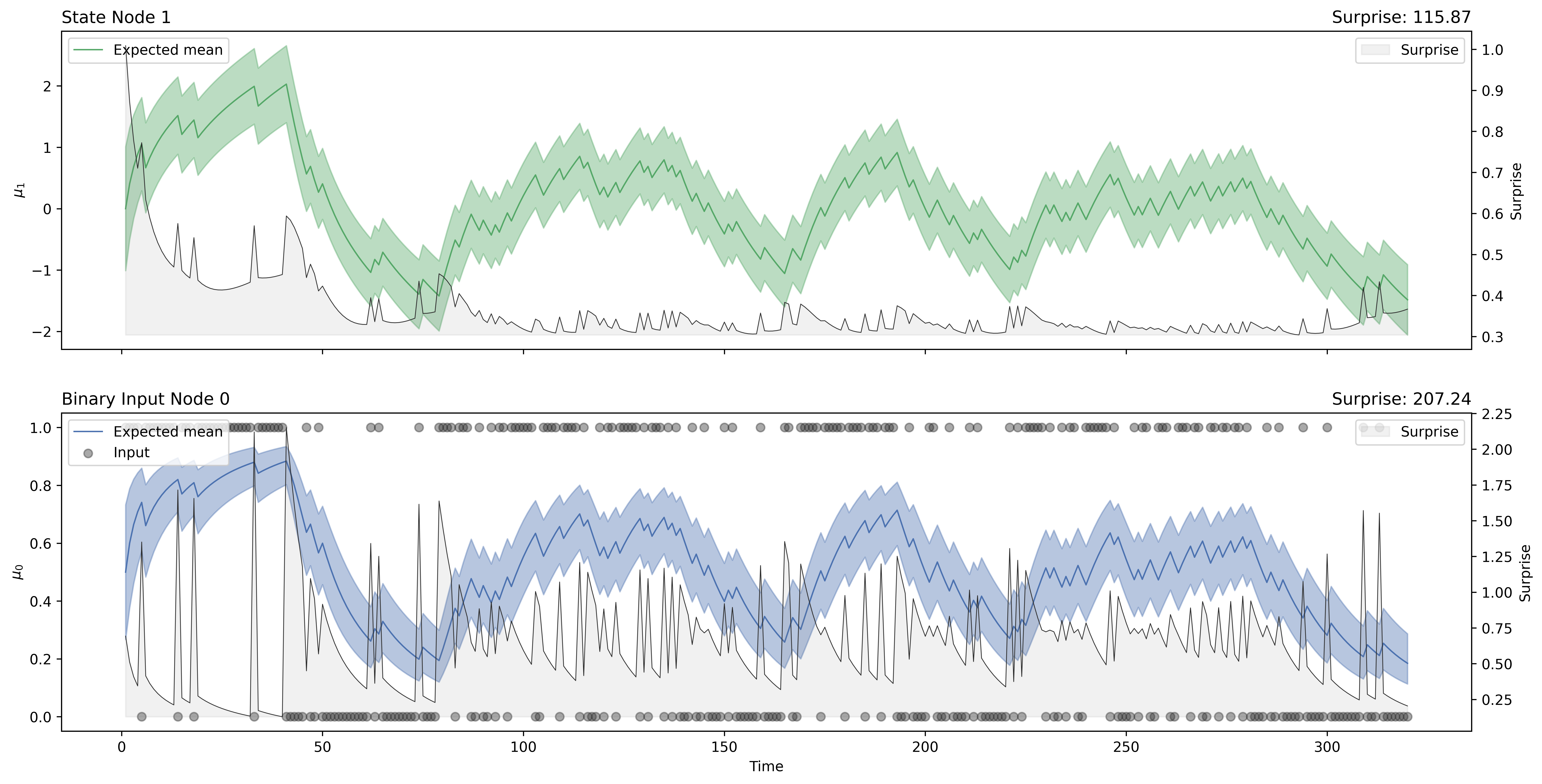
Here we demonstrate how to fit forwards a two-level binary Hierarchical Gaussian filter. The input time series are binary observations using an associative learning task Iglesias et al. (2013).

from pyhgf.model import Network
from pyhgf import load_data

# Load time series example data (observations, decisions)
u, y = load_data("binary")

# Create a two-level binary HGF from scratch
hgf = (
    Network()
    .add_nodes(kind="binary-state")
    .add_nodes(kind="continuous-state", value_children=0)
)

# add new observations
hgf.input_data(input_data=u)

# visualization of the belief trajectories
hgf.plot_trajectories();

from pyhgf.response import binary_softmax_inverse_temperature

# compute the model's surprise (-log(p)) 
# using the binary softmax with inverse temperature as the response model
surprise = hgf.surprise(
    response_function=binary_softmax_inverse_temperature,
    response_function_inputs=y,
    response_function_parameters=4.0
)
print(f"Sum of surprises = {surprise.sum()}")

Model's surprise = 138.8992462158203

Acknowledgments

This implementation of the Hierarchical Gaussian Filter was inspired by the original Matlab HGF Toolbox. A Julia implementation is also available here.

References

1. Legrand, N., Weber, L., Waade, P. T., Daugaard, A. H. M., Khodadadi, M., Mikuš, N., & Mathys, C. (2024). pyhgf: A neural network library for predictive coding (Version 1). arXiv. https://doi.org/10.48550/ARXIV.2410.09206
2. Mathys, C. (2011). A Bayesian foundation for individual learning under uncertainty. In Frontiers in Human Neuroscience (Vol. 5). Frontiers Media SA. https://doi.org/10.3389/fnhum.2011.00039
3. Mathys, C. D., Lomakina, E. I., Daunizeau, J., Iglesias, S., Brodersen, K. H., Friston, K. J., & Stephan, K. E. (2014). Uncertainty in perception and the hierarchical Gaussian filter. Frontiers in Human Neuroscience, 8. https://doi.org/10.3389/fnhum.2014.00825
4. Weber, L. A., Waade, P. T., Legrand, N., Møller, A. H., Stephan, K. E., & Mathys, C. (2023). The generalized Hierarchical Gaussian Filter (Version 2). arXiv. https://doi.org/10.48550/ARXIV.2305.10937
5. Frässle, S., Aponte, E. A., Bollmann, S., Brodersen, K. H., Do, C. T., Harrison, O. K., Harrison, S. J., Heinzle, J., Iglesias, S., Kasper, L., Lomakina, E. I., Mathys, C., Müller-Schrader, M., Pereira, I., Petzschner, F. H., Raman, S., Schöbi, D., Toussaint, B., Weber, L. A., … Stephan, K. E. (2021). TAPAS: An Open-Source Software Package for Translational Neuromodeling and Computational Psychiatry. In Frontiers in Psychiatry (Vol. 12). Frontiers Media SA. https://doi.org/10.3389/fpsyt.2021.680811
6. Iglesias, S., Kasper, L., Harrison, S. J., Manka, R., Mathys, C., & Stephan, K. E. (2021). Cholinergic and dopaminergic effects on prediction error and uncertainty responses during sensory associative learning. In NeuroImage (Vol. 226, p. 117590). Elsevier BV. https://doi.org/10.1016/j.neuroimage.2020.117590