Orbit Simulator

Overview

There use to be a nifty orbit simulator for Mac Sytem 6 or so. It let users input an arbitrary system, then it would simulate how the planets and stars would orbit each other. It was all black and white, and was rather limited. But it was always fun to try and create the most complicated but stable system you could. I remember this program fondly, but can't find it anywhere. Nor can I find such an easy to use simulator like it.

This is my attempt to create an orbit simulator that is intuitive, easy to use and fun, while remaining as accurate as possible.

Features

Full N-body simulation in Javascript
Three different algorithms to choose from
Play, pause and reset a simulation
Record a simulation to an animated GIF
Accelerate simulation either by calculating more between frames (accurate, but slower), or by skipping more time (less accurate, but fast)
Save a simulation to your browser's Local Storage
Save and reload a simulation via JSON files
Export positional data to CSV for analysis
Touch accessible
A number of presets demonstrating capibilities
Calculate Lagrange points (approximatly)
Generate random objects to simulate evalution of a system
Collisions between objects

Details

This simulator implements three different iterative algorithms to simulate gravity. By default, we use Runge-Kutta, as it has shown to be much more stable than Euler or Verlet, with only a small speed difference.

The code supports a 3D simulation, but display an input are limited to 2 dimentions at this time.

By default, new objects are created at the distance from the center that was clicked, and given a speed to make a circular orbit, assuming a single star at the center point as the first object. Values can be modified to suite, but this seemed like a good estimate to start.

It is capable of storing the current state into your browser's Local Storage, or exporting to a JSON file. You can then choose to load the state or setup from either the last local store, or a selected JSON file. State loads all the history and places the object at the last location. Setup loads the objects and places them in their initial locations without history. Note that no data is sent for either local storage or file storage to a remote server. All remains local to your browser.

Science

Gravitation

This simulation works by iteritivly calculating the forces on objects. Universal Gravitation says that:

$F = G \frac{M_{1}+M_{2}}{r^{2} }$

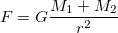
where G is the gravitational constant, M1 and M2 are masses being attacted, and r is the distance between them. Newton's second law also says:

$F=M_{1}a$

$a = \frac{F}{M_{1}}$

so we know that the force acting on an object changes the acceleration based on the mass of the object. Therefore

$a = G \frac{M_{2}}{ r^{2} }$

which means that the acceleration experinced by an object is based on the mass of the other object divided by the square of the distance between them, multiplied by a constant. Do this for every object acting on the current one, and you have the new acceleration. Update the position and velocity based on the time between calculations.

Additionally, because the gravitational constant G is very very small, and most values in space are very very very big, values here have been scaled by G to reduce the computation needed, and the deal in smaller numbers. They are still really big, so things where scaled again further shrink numbers without loosing accuracy. So don't use these numbers to launch a space ship, or do your homework.

Easy, right?

Simulation

The trick is the acculated error from large enough time steps. There are three methods considered for this simulator:

Euler
- Simple, just do the calculation at every step
- $v_1 = a_1 * \Delta t x_1 = v_1 * \Delta t$
Verlet
- Estimates a half way value to correct for some error
- First iteration bootstraps based on velocity, while the rest just use the previous position
- $x_1 = x_0 = v_0 \Delta t + \frac{1}{2} a \Delta t^2 x_{n} = 2 * x_{n-1} - x_{n-2} + a \Delta t^2$
Runge-Kutta
- Estimates, based on differential equations, 4 sub steps, to correct for more error
- $x_{rk1} = x_{n-1} v_{rk1} = v_{n-1}$
- $x_{rk2} = v_{rk1} \frac{1}{2} \Delta t + x_{n-1} v_{rk2} = accel(x_{rk1}) \frac{1}{2} \Delta t + v_{n-1}$
- $x_{rk3} = v_{rk2} \frac{1}{2} \Delta t + x_{n-1} v_{rk3} = accel(x_{rk2}) \frac{1}{2} \Delta t + v_{n-1}$
- $x_{rk4} = v_{rk3} \Delta t + x_{n-1} v_{rk4} = accel(x_{rk3}) \Delta t + v_{n-1}$
- $x_n = \frac {1}{6} \left( v_{rk1} + 2v_{rk2} + 2v_{rk3} + v_{rk4} \right) v_n = \frac {1}{6} \left( accel(x_rk1) + 2accel(x_{rk2}) + 2accel(x_{rk3}) + accel(x_{rk4}) \right)$
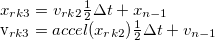
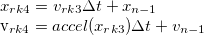
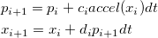
- where accel(x) is the acceleration of the object being considered at point x at the current time.
Symplectic Integration
- Alternates between computing position and momentum, to keep energy constant
- Available in 1st, 2nd, 3rd, and 4th order varients, depending on number of coeffients
- $\begin{pmatrix}c_1, c_2, ... \\d_1, d_2, ...\end{pmatrix}$
- $\begin{align*}& p_{i+1} = p_i + c_i accel(x_i) dt \\& x_{i+1} = x_i + d_i p_{i+1} dt\end{align*}$
- First order is just Euler above
- Second order: $\begin{pmatrix}0& 1\\1/2& 1/2 \end{pmatrix}$
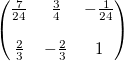
- Third order: $\begin{pmatrix}\frac{7}{24} & \frac{3}{4} & -\frac{1}{24}\\ \\ \frac{2}{3} & -\frac{2}{3} & 1 \end{pmatrix}$
- Fourth order: $\frac{1}{2-\sqrt[3]{2}} \begin{pmatrix}\frac{1}{2} & \frac{1 - \sqrt[3]{2}}{2} & \frac{1 - \sqrt[3]{2}}{2} & \frac{1}{2}\\ \\0 & 1 & -\sqrt[3]{2} & 1\end{pmatrix}$

This simulator defaults to Verlet, as it is fast, and reasonably accurate. While RK and Ruth should be more accurate, they seem to accumlate percision error much faster.

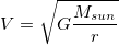
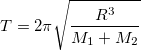
Orbital velocity

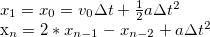
When adding a new object, the panel is initialized with a resonable first guess of a circular orbit. This is because the velocity of a circular orbit is approximatly:

$V = \sqrt{G \frac{M_{sun}}{r}}$

Lagrange

Lagrange points are simi-stable orbits that remain fixed in reference to a primary and secondary (sun and planet, planet and moon) object. At these points, the gravitation of the two objects, combined with the cretrifgual force experienced in orbit, cancel each other out. These are approximatly on either side of the secondary object inline with the primary (L1 and L2), in the opposite side of the secondary's orbit (L3), and at 60 degrees ahead and behind the secondary's orbit (L4 and L5).

The full derivation becomes quite complicated and results in a 5th order equation that can't be generally solved. So either estimates are made, assuming the secondary object is much smaller than the primary, or it is solved iterativly, searching for these equalibrium points with finer and finer grain passes. This simulator uses the second approach.

L4 and L5 are trivial to calculate, as they are at the same disance from the barrycenter as the secondary, and in the same orbit, just offset by 60 degrees either side.

The primary orbits the barrycenter at

$r_{1} = R \frac{M_{2}}{M_{1} + M_{2}}$

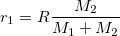
Using that, you can calculate the distance from both the primary and secondary objects, depending on which point you want to solve for, with L1 being between primary and secondary, L2 being near the secondary but with both primary and secondary on the same side, and L3 being on the opposite side of the primary from the secondary.

The gravitation experienced at each of these points depends on which point to consider, some adding and some subtracting, but the base is the same, so we'll consider the L1 point.

$F_g = G\frac{M_1}{r_1^2} - G\frac{M_2}{r_2^2}$

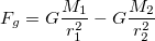
that is, the gravitational force of the primary, minus the gravitational force of the secondary. For L2 and L3, the forces add.

The object also has centrifigual forces, as it orbits, based on it's speed. As the object short orbit in the same period as the secondary, we can calculate speed for the proposed orbit.

$T = 2 \pi \sqrt{\frac{R^3}{M_1 + M_2}}$

$v = 2 \pi \frac{r}{T}$

$F_c = \frac{v^2}{r}$

To solve for the proper radius, itterativly propose a radius, and find out when the forces over balance, and then try again, with a smaller step, until you find approximatly 0 difference. Then you have your solution. Much easier than solving this:

$\vec{F_\Omega} = 0 = \Omega^2\left(x - \frac{\beta(x + \alpha R)R^3}{((x+\alpha R)^2 + y^2)^{3/2}} - \frac{\alpha (x-\beta R)R^3}{((x-\beta R)^2 + y^2)^{3/2}}\right)\hat{i} + \Omega^2\left(y - \frac{\beta y R^3}{((x+\alpha R)^2 + y^2)^{3/2}} - \frac{\alpha yR^3}{((x-\beta R)^2 + y^2)^{3/2}}\right)\hat{j}$

jdiwnab / OrbitSim

readme