 teorth
commented
5 years ago
teorth
commented
5 years ago Thanks for this - it's easy for me to step through it myself now. The multiplicative factor for 317 should have N^(-(1+I*xt)\/2) rather than N^((1+I*xt)\/2)\/8 (I guess the 1\/8 factor was just dropped at the very start, as it wasn't important), which seems to fix that step at least.
Similarly, the multiplicative factor for 318 should be N^(-(1+I*xt)\/2)*sqrt(Pi\/(1-Iu\/(8*Pi))) rather than N^((1+I*xt)/2)/8\sqrt(Pi) .
Now checking 3.20...
 rudolph-git-acc
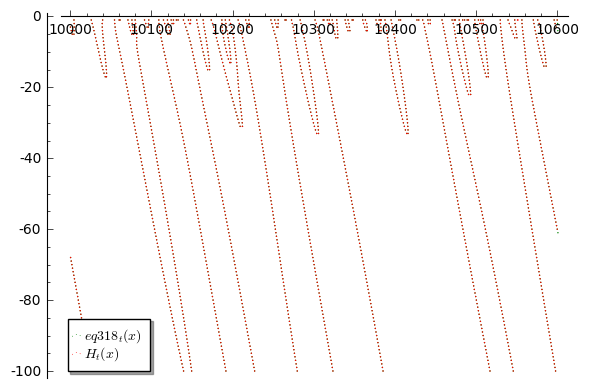
 km-git-acc
 p15-git-acc


Grateful for any help to properly evaluate the sequence of equations on this Wiki page: http://michaelnielsen.org/polymath1/index.php?title=Polymath15_test_problem#Large_negative_values_of_.5Bmath.5Dt.5B.2Fmath.5D
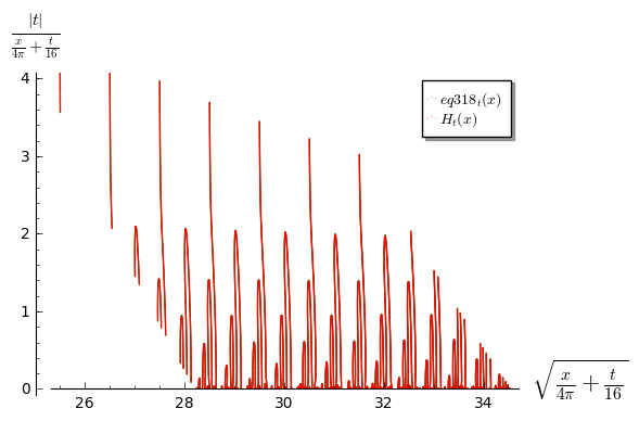
Below is the pari/gp code I have used so far. At the end of the code is a simple rootfinder that should (approximately) find this sequence of roots:
however from eq 318 onwards it finds many more roots (also at different t, e.g. -100). Have experimented with the integral limits, the integral's fixed parameter, the real precision settings of pari and the size of the sums, but no success yet.
Have re-injected some of the non-zero multiplication factors that can be switched on/off if needed.
One thing I noticed is that after eq 307 the function doesn't seem to be real anymore (see data at the end). Not sure if this should matter though, since I use the real value of Ht for root finding.