Help need for evaluation of latest wiki page equations

[rudolph-git-acc]

Grateful for any help to properly evaluate the sequence of equations on this Wiki page: http://michaelnielsen.org/polymath1/index.php?title=Polymath15_test_problem#Large_negative_values_of_.5Bmath.5Dt.5B.2Fmath.5D

Below is the pari/gp code I have used so far. At the end of the code is a simple rootfinder that should (approximately) find this sequence of roots:

-10.00000000, 906.72649548
-10.00000000, 931.47009390
-10.00000000, 976.80075639
-10.00000000, 990.45190417

however from eq 318 onwards it finds many more roots (also at different t, e.g. -100). Have experimented with the integral limits, the integral's fixed parameter, the real precision settings of pari and the size of the sums, but no success yet.

Have re-injected some of the non-zero multiplication factors that can be switched on/off if needed.

One thing I noticed is that after eq 307 the function doesn't seem to be real anymore (see data at the end). Not sure if this should matter though, since I use the real value of Ht for root finding.

default(realprecision, 40)

Xi(s)=return((s/2)*(s-1)*Pi^(-s/2)*gamma(s/2)*zeta(s));
M0(s)=return(s*(s-1)/2*Pi^(-s/2)*sqrt(2*Pi)*exp((s/2-1/2)*log(s/2)-s/2));

Ht302(x,t) = {
    A=intnum(v=-8,8,Xi((1+I*x)/2+I*sqrt(abs(t))*v)*exp(-v^2),1);
    return(A);
}

Ht303(x,t) = {
    A=intnum(v=-8,8,Xi((1+I*x)/2+I*sqrt(abs(t))*v-Pi*I*abs(t)/8)*exp(-(v-Pi*sqrt(abs(t))/8)^2),1);
    return(A);
}

Ht304(x,t) = {
    xt = x-Pi*abs(t)/4;
    mulfact = exp(-Pi^2*abs(t)/64);
    A=mulfact*intnum(v=-8,8,Xi((1+I*xt)/2+I*sqrt(abs(t))*v)*exp(-v^2+Pi*sqrt(abs(t))*v/4),1);
    return(A);
}

Ht307(x,t) = {
    xt = x-Pi*abs(t)/4;
    mulfact = exp(-Pi^2*abs(t)/64)*2;
    A=mulfact*intnum(v=-8,8,real(M0((1+I*xt)/2+I*sqrt(abs(t))*v))*zeta((1+I*xt)/2+I*sqrt(abs(t))*v)*exp(-v^2+Pi*sqrt(abs(t))*v/4),1);
    return(A);
}

Ht312(x,t) = {
    xt = x-Pi*abs(t)/4;
    mulfact = exp(-Pi^2*abs(t)/64)*(M0((1+I*xt)/2));
    A= mulfact*intnum(v=-8,8,exp((I*sqrt(abs(t))*v)/2*log(xt/(4*Pi))-Pi*sqrt(abs(t))*v/4+(I*abs(t)*v^2)/(2*xt))*zeta((1+I*xt)/2+I*sqrt(abs(t))*v)*exp(-v^2+Pi*sqrt(abs(t))*v/4),1);
    return(A);
}

Ht315(x,t) = {
    xt = x-Pi*abs(t)/4;
    N = sqrt(xt/(4*Pi));
    u = 4*Pi*abs(t)/xt;
    mulfact = exp(-Pi^2*abs(t)/64)*(M0((1+I*xt)/2));
    A=mulfact*intnum(v=-8,8,exp(I*sqrt(abs(t))*v*log(N)+I*u*v^2/(8*Pi))*zeta((1+I*xt)/2+I*sqrt(abs(t))*v)*exp(-v^2),1);
    return(A);
}

Ht316(x,t) = {
    xt = x-Pi*abs(t)/4;
    N = sqrt(xt/(4*Pi));
    u = 4*Pi*abs(t)/xt;
    mulfact = exp(-Pi^2*abs(t)/64)*(M0((1+I*xt)/2));
    A=mulfact*sum(n=1,1000, intnum(v=-8,8,exp(I*sqrt(abs(t))*v*log(N)+I*u*v^2/(8*Pi))*n^(-((1+I*xt)/2+I*sqrt(abs(t))*v))*exp(-v^2),1));
    return(A);
}

Ht317(x,t) = {
    xt = x-Pi*abs(t)/4;
    N = sqrt(xt/(4*Pi));
    u = 4*Pi*abs(t)/xt;
    mulfact = exp(-Pi^2*abs(t)/64)*(M0((1+I*xt)/2))*N^((1+I*xt)/2)/8;
    A=mulfact*sum(n=1,1000, intnum(v=-8,8,exp(-I*sqrt(abs(t))*v*log(n/N)+I*u*v^2/(8*Pi)-((1+I*xt)/2)*log(n/N))*exp(-v^2),1));
    return(A);
}

Ht318(x,t) = {
    xt = x-Pi*abs(t)/4;
    N = sqrt(xt/(4*Pi));
    u = 4*Pi*abs(t)/xt;
    mulfact = exp(-Pi^2*abs(t)/64)*(M0((1+I*xt)/2))*N^((1+I*xt)/2)/8*sqrt(Pi);
    A=mulfact*sum(n=1,1000,exp(-abs(t)*(log(n/N))^2/(4*(1-I*u/(8*Pi)))-(1+I*xt)/2*log(n/N)));
    return(A);
}

Ht320(x,t) = {
    xt = x-Pi*abs(t)/4;
    N = sqrt(xt/(4*Pi));
    u = 4*Pi*abs(t)/xt;
    mulfact = exp(-Pi^2*abs(t)/64)*(M0((1+I*xt)/2))*N^((1+I*xt)/2)/8*sqrt(Pi);
    A = mulfact*sum(n=1,1000,exp(-(abs(t)*(n-N)^2)/(4*N^2*(1-I*u/(8*Pi)))-I*xt/2*(n-N)/N+I*xt*(n-N)^2/(4*N^2)));
    return(A);
}

Ht321(x,t) = {
    xt = x-Pi*abs(t)/4;
    N = sqrt(xt/(4*Pi));
    u = 4*Pi*abs(t)/xt;
    mulfact = exp(-Pi^2*abs(t)/64)*(M0((1+I*xt)/2))*N^((1+I*xt)/2)/8*sqrt(Pi);
    A = mulfact*sum(n=1,1000,exp(-(2*Pi*u*(n-N)^2)/(8*Pi-I*u)-2*Pi*I*N*(n-N)+Pi*I*(n-N)^2));
    return(A);
}

Ht323(x,t) = {
    xt = x-Pi*abs(t)/4;
    N = sqrt(xt/(4*Pi));
    u = 4*Pi*abs(t)/xt;
    mulfact = exp(-Pi^2*abs(t)/64)*(M0((1+I*xt)/2))*N^((1+I*xt)/2)/8*sqrt(Pi);
    A = mulfact*sum(n=1,1000,exp(-(2*Pi*u*(n-N)^2)/(8*Pi-I*u)-Pi*I*n^2+2*Pi*I*(n-N)^2));
    return(A);
}

Ht324(x,t) = {
    xt = x-Pi*abs(t)/4;
    N = sqrt(xt/(4*Pi));
    u = 4*Pi*abs(t)/xt;
    mulfact = exp(-Pi^2*abs(t)/64)*(M0((1+I*xt)/2))*N^((1+I*xt)/2)/8*sqrt(Pi);
    A = mulfact*sum(n=1,1000,exp((16*Pi^2*I*(n-N)^2)/(8*Pi-I*u))*exp(Pi*I*n));
    return(A);
}

Ht328(x,t) = {
    xt = x-Pi*abs(t)/4;
    N = sqrt(xt/(4*Pi));
    u = 4*Pi*abs(t)/xt;
    mulfact = exp(-Pi^2*abs(t)/64)*(M0((1+I*xt)/2))*N^((1+I*xt)/2)/8*sqrt(Pi);
    A = mulfact*sum(n=1,1000,exp(-Pi*I*n*(n+1)/2)*exp(2*Pi*I*(n+1/2)*N)*exp(-u*n*(n+1)/16));
    return(A);
}

print("eq.302 ",Ht302(1000, -10))
print("eq.303 ",Ht303(1000, -10))
print("eq.304 ",Ht304(1000, -10))
print("eq.307 ",Ht307(1000, -10))
print("eq.315 ",Ht315(1000, -10))
print("eq.316 ",Ht316(1000, -10))
print("eq.317 ",Ht317(1000, -10))
print("eq.318 ",Ht318(1000, -10))
print("eq.320 ",Ht320(1000, -10))
print("eq.321 ",Ht321(1000, -10))
print("eq.323 ",Ht323(1000, -10))
print("eq.324 ",Ht324(1000, -10))
print("eq.328 ",Ht324(1000, -10))

xs = 900; xe = 1010;
ts = -10; te = -1;
f=Ht318;
forstep(t=ts, te, 10, {
    xc = xs;
    while(xc <= xe,
        if(real(f(xc,t))*real(f(xc+1,t)) < 0, root=solve(a=xc, xc+1, real(f(a,t))); printf("%3.8f, %3.8f\n",t, root));
        xc=xc+1);
})

eq.302 1.201485926838305713580758240853488704456 E-165 + 3.514303326279329051 E-221*I
eq.303 1.201485926838305713582303927841938470920 E-165 + 3.522103826014908131 E-221*I
eq.304 1.201485926838305713582303927841938470920 E-165 + 3.522103826014922598 E-221*I
eq.307 1.201477416607903787215861199656638682224 E-165 + 3.992587328505261451855248837227037420869 E-169*I
eq.312 1.200242494404236645648308584282451391036 E-165 + 4.014384445003979486997306873566995218158 E-169*I
eq.315 1.200242494404236645648308584282451391036 E-165 + 4.014384445003979486997306873566995218158 E-169*I
eq.316 1.200242494404236645648308630967087228353 E-165 + 4.014384445003979487000178658198142256762 E-169*I
eq.317 1.210630457223022714918883693478442584040 E-165 - 5.581422172204223838770738013241198104262 E-166*I
eq.318 1.209227903617935860382758702133562335051 E-165 - 5.611945144292097211229689587084475461023 E-166*I
eq.320 2.791674127351571571455964690537038072397 E-167 - 2.126109533152847673586778474944806978351 E-167*I
eq.321 2.791674127351571571455964690537038072397 E-167 - 2.126109533152847673586778474944806978351 E-167*I
eq.323 -3.076893561828845392623560432368639943370 E-167 + 1.687160985046708488717820653125387727510 E-167*I
eq.324 -3.076893561828845392623560432368639943370 E-167 + 1.687160985046708488717820653125387727510 E-167*I
eq.328 -3.076893561828845392623560432368639943370 E-167 + 1.687160985046708488717820653125387727510 E-167*I

[rudolph-git-acc]

Let me play back to ensure I fully understood. I have written 1.18 fully in N, u and capped u at 4 as follows:

Ht118f(N,t) = {
    u = if(4*Pi*abs(t)/(4*Pi*N^2)<4,4*Pi*abs(t)/(4*Pi*N^2), 4);
    mulfact = exp(Pi^2*(-u*N^2)/64)*(M0((1+I*(4*Pi*N^2))/2))*N^(-(1+I*(4*Pi*N^2))/2)/(8*sqrt(1-I*u/(8*Pi)));
    A=mulfact*sum(n=1,1000,exp(-u*(n-N)^2/(4*(1-I*u/(8*Pi)))-2*Pi*I*N^2*log(n/N)));
    return(A);
}

When I then run the root finding for N[26, 34], t [-3000,-2980], I do get roots at approximately half an integer like these:

-3000.00000000, 26.50506056
-3000.00000000, 27.50506039
-3000.00000000, 28.50646986
-3000.00000000, 29.50802722
-3000.00000000, 30.50974867
-3000.00000000, 31.51165483
-3000.00000000, 32.51377237
-3000.00000000, 33.51613622
-3000.00000000, 34.51879268
-2990.00000000, 26.50506056
-2990.00000000, 27.50513046
-2990.00000000, 28.50655129
-2990.00000000, 29.50812153
-2990.00000000, 30.50985767
-2990.00000000, 31.51178081
-2990.00000000, 32.51391822
-2990.00000000, 33.51630570
-2990.00000000, 34.51899072
-2980.00000000, 26.50506056
-2980.00000000, 27.50520138
-2980.00000000, 28.50663372
-2980.00000000, 29.50821699
-2980.00000000, 30.50996805
-2980.00000000, 31.51190842
-2980.00000000, 32.51406604
-2980.00000000, 33.51647757
-2980.00000000, 34.51919170

The same, but now for N[100, 110], t [-3000,-2980]

-3000.00000000, 100.42704250
-3000.00000000, 101.42812900
-3000.00000000, 102.42922063
-3000.00000000, 103.43031384
-3000.00000000, 104.43140573
-3000.00000000, 105.49725631
-3000.00000000, 106.43357639
-3000.00000000, 107.99954423
-3000.00000000, 109.17267055
-3000.00000000, 110.17303455
-2990.00000000, 100.42706678
-2990.00000000, 101.42815533
-2990.00000000, 102.42924850
-2990.00000000, 103.43034285
-2990.00000000, 104.43143553
-2990.00000000, 105.49729523
-2990.00000000, 106.43360700
-2990.00000000, 107.99958021
-2990.00000000, 109.17270673
-2990.00000000, 110.17306971
-2980.00000000, 100.42709133
-2980.00000000, 101.42818186
-2980.00000000, 102.42927653
-2980.00000000, 103.43037196
-2980.00000000, 104.43146540
-2980.00000000, 105.49733403
-2980.00000000, 106.43363763
-2980.00000000, 107.99961606
-2980.00000000, 109.17274278
-2980.00000000, 110.17310474

No longer at the half integer, but the vertical line pattern clearly remains.

EDIT: and for N[10000, 10010], t [-3000,-2980]. Seems that rationals are preferred.

-3000.00000000, 10001.74999702
-3000.00000000, 10004.99999730
-3000.00000000, 10005.12499807
-3000.00000000, 10009.40234201
-3000.00000000, 10010.99999869
-2990.00000000, 10001.74999702
-2990.00000000, 10004.99999731
-2990.00000000, 10005.12499808
-2990.00000000, 10009.40234201
-2990.00000000, 10010.99999867
-2980.00000000, 10001.74999703
-2980.00000000, 10004.99999733
-2980.00000000, 10005.12499808
-2980.00000000, 10009.40234200
-2980.00000000, 10010.99999865

Before I run any plots, is this what you are after?

[p15-git-acc]

Here's a table for f_m in 1.31 with integration limits [1, 1000]. Until this has been separately verified it doesn't deserve too much confidence.

N	u	m	f
25	1	0.5	6.064170622e-67 + 7.002959331e-67*i
25	1	-0.5	6.054434829e-67 + 6.99179685e-67*i
25	1	1.5	6.073937786e-67 + 7.014157503e-67*i
25	1	-1.5	6.044730254e-67 + 6.980669889e-67*i
25	2	0.5	-1.153538163e-128 + 6.175333684e-129*i
25	2	-0.5	-1.151699671e-128 + 6.165335326e-129*i
25	2	1.5	-1.155382533e-128 + 6.185364533e-129*i
25	2	-1.5	-1.149867029e-128 + 6.155369301e-129*i
30	1	0.5	1.207083633e-95 - 1.601587694e-97*i
30	1	-0.5	1.205743102e-95 - 1.599418532e-97*i
30	1	1.5	1.208427149e-95 - 1.60376261e-97*i
30	1	-1.5	1.204405544e-95 - 1.597255099e-97*i
30	2	0.5	5.834234793e-186 + 1.289560178e-186*i
30	2	-0.5	5.82774568e-186 + 1.28816291e-186*i
30	2	1.5	5.840738373e-186 + 1.290960476e-186*i
30	2	-1.5	5.821270985e-186 + 1.286768663e-186*i
35	1	0.5	-1.037500738e-130 - 6.241105659e-130*i
35	1	-0.5	-1.036641524e-130 - 6.236014631e-130*i
35	1	1.5	-1.038361377e-130 - 6.246205006e-130*i
35	1	-1.5	-1.035783734e-130 - 6.230931902e-130*i
35	2	0.5	-7.709124659e-255 + 4.628822016e-254*i
35	2	-0.5	-7.703007672e-255 + 4.625040768e-254*i
35	2	1.5	-7.715251353e-255 + 4.632609451e-254*i
35	2	-1.5	-7.696900368e-255 + 4.621265693e-254*i

[teorth]

Let me play back to ensure I fully understood. I have written 1.18 fully in N, u and capped u at 4 as follows:

Ht118f(N,t) = {
    u = if(4*Pi*abs(t)/(4*Pi*N^2)<4,4*Pi*abs(t)/(4*Pi*N^2), 4);
    mulfact = exp(Pi^2*(-u*N^2)/64)*(M0((1+I*(4*Pi*N^2))/2))*N^(-(1+I*(4*Pi*N^2))/2)/(8*sqrt(1-I*u/(8*Pi)));
    A=mulfact*sum(n=1,1000,exp(-u*(n-N)^2/(4*(1-I*u/(8*Pi)))-2*Pi*I*N^2*log(n/N)));
    return(A);
}

Well, I was thinking of making (N,u) the variables rather than (N,t) and then one can delete the first line of code, but yeah, that's basically what I had in mind. (One should first check that one recovers the original plot of zeroes in the range u in [0,4], N in [26,34] that you previously had by this method, of course).

[rudolph-git-acc]

Thanks, got it now. Here is the test plot for u[0,4] (step 0.1), [26,34] (step 1):

Plot for u[0,4] (step 0.1), [100,110] (step 0.1):

[teorth]

p15: Thanks for the preliminary data! It is strange to me that the output is more or less even in m (replacing m by -m gives almost the same output). I was expecting the output for -m to be approximately the complex conjugate of that for m, as things have to sum to be approximately real. Not sure what to make of that yet.

[teorth]

Rudolph: if I am understanding your plot correctly, is the test plot only capturing some but not all of the zeroes of H_t? Because some of the red loops don't have any green dots on them. That's bizarre to me, in particular the jump in the green dots to the right around u=1.4 seems "wrong" somehow. Does locating the zeroes of 1.18 in the original t, coordinates reproduce the red curves? If so the issue must be some strange interaction between the zero finding algorithm and the change of coordinates.

EDIT: it may help to work with the normalised multiplier mulfact/abs(mulfact) rather than mulfact in order to avoid artefacts arising from rapidly changing magnitudes.

[rudolph-git-acc]

I think this is purely caused by the step size I used for test run (i.e. I don't capture all zeros). Have just added [100, 110] with smaller step size for N (0.1) but that's not good enough. Will let [200, 210] run overnight in a higher resolution for N.

[rudolph-git-acc]

Have applied the normalised multiplier (was indeed needed) and switched to the standard implicit plots, which are faster to produce. Could boost the resolution further if needed.

N[26, 34], t[0, 4] (n=100)

N[100, 110], t[0, 4] (n=200)

N[200, 210], t[0, 4] (n=300)

N[600, 610], t[0, 4] (n=700)

[teorth]

Ah! It's beginning to make more sense now. These periodic patterns we are seeing are coming somehow from the higher order terms in the Taylor expansion, but die out as N goes to infinity at which point the theta function asymptotics finally take over and one just gets the boring parallel lines. In particular they're not actually fully periodic in N, they are also decaying in u. That's why I couldn't get a good explanation for these little loops; in the asymptotic regime I was working with, in which I was basically holding u fixed and sending N to infinity, the loops disappear. Very roughly it looks like the interesting regime may instead be when u decays something like N^{-1/2} or maybe N^{-1/3} (can't tell really at this point without a bit more data). But now I have better guidance on how to do the asymptotics...

[p15-git-acc]

I can reproduce the last three of Rudolph's implicit plots, with 1000 summation terms.

N in [100, 110]:

N in [200, 210]:

N in [600, 610]:

[p15-git-acc]

Zooming in on N[600, 602], u[0, 1] with 1000 summation terms:

[teorth]

Beautiful! It's interesting that now there is a 1/2-periodicity rather than a 1-periodicity that is beginning to emerge.

For the final zoomed in plot, could you try replacing the final factor of log(n/N) in 1.18 with two or more terms of the Taylor expansion and see what happens to the picture? That is, to use the approximations

(n-N)/N - (n-N)^2 / (2*N^2)

(n-N)/N - (n-N)^2 / (2*N^2) + (n-N)^3 / (3*N^3)

(n-N)/N - (n-N)^2 / (2*N^2) + (n-N)^3 / (3*N^3) - (n-N)^4 / (4*N^4)

for log(n/N).

[p15-git-acc]

This table shows approximately how the maximum size of u at which interesting roots of the real part of 1.18 are found decays as a function of N.

N	u
40	1.8046875
60	1.5546875
80	1.3984375
100	1.2734375
120	1.1953125
140	1.1171875
160	1.0546875
180	1.0078125
200	0.9609375
220	0.9140625
240	0.8828125
260	0.8515625
280	0.8203125
300	0.8046875
320	0.7734375
340	0.7578125
360	0.7421875
380	0.7265625
400	0.7109375
420	0.6953125
440	0.6796875
460	0.6640625
480	0.6484375
500	0.6328125
520	0.6328125
540	0.6171875
560	0.6015625
580	0.6015625
600	0.5859375
620	0.5859375
640	0.5703125
660	0.5703125
680	0.5546875
700	0.5546875
720	0.5390625
740	0.5390625
760	0.5234375
780	0.5234375
800	0.5234375
820	0.5078125
840	0.5078125
860	0.4921875
880	0.4921875
900	0.4921875
920	0.4765625
940	0.4765625
960	0.4765625
980	0.4765625
1000	0.4609375

[p15-git-acc]

Second order Taylor expansion of final factor of log(n/N) in 1.18:

Third order Taylor expansion of final factor of log(n/N) in 1.18:

Fourth order Taylor expansion of final factor of log(n/N) in 1.18:

The solid green in the second order expansion might mean that the calculation yields an interval that includes zero or maybe there is something going on with non negligible imaginary parts, or maybe it's just riddled with zeros of the real part. I haven't looked at it in detail.

[rudolph-git-acc]

Did a quick check on N[1000, 1002], u[0, 1] and do get the same 'solid green' effect in the second order expansion.

Using log(n/N):

Second order expansion of log(n/N) = (n-N)/N - (n-N)^2 / (2*N^2):

Third order expansion of log(n/N) = (n-N)/N - (n-N)^2 / (2N^2) + (n-N)^3 / (3N^3)

[teorth]

Thanks for this! So now we are in a region where the third order Taylor expansion has started to work again. Now that I know that u is supposed to be small rather than large, I realise that I had been doing Poisson summation inefficiently. I've redone that calculation in the wiki and now think I have a better approximation that should start clarifying the situation.

Would it be possible for one or both of you to plot (in the same region u in [0,1], N in [1000,1002] as in the above image the zeroes of:

• The equation (1.20) (this should be identical to the final plot of Rudolph's, but this is just to double check)

• The equation (1.40) (this should be identical to (1.20))

• The equation (1.41) (it should be safe for m to range in something like -10..10, and in (1.42) X should be able to range in something like [N-100, N+100] (or [-100,100] for (1.43)). If the zeroes are problematic to locate for this equation then just a comparative plot or table of the values of (1.40) and (1.41) at some test values of N,u would be helpful. Also a table of the first few values of g_m to get some idea of how fast they drop in size. I'm hoping that just the m=0,1 values are dominant as then one just has to analyse the integrals g_0, g_1 which are Airy functions (and now that I look at it, the asymmetric oscillations we are seeing here are a little bit reminiscent of how the Airy function looks: https://en.wikipedia.org/wiki/Airy_function )

[teorth]

p15: Hmm, a log log plot of your N, u data suggests a relation roughly of the form u^(5/2) ~ 150/N, which is not a relationship I was expecting. The exponent 5/2 is a bit strange, it suggests that at some point a fairly high Taylor expansion in u (or u^{1/2}) will come into play...

[p15-git-acc]

Very roughly it looks like the interesting regime may instead be when u decays something like N^{-1/2} or maybe N^{-1/3} (can't tell really at this point without a bit more data).

Fitting this table I get about u = a*N^b + c where

a = 7.152
b = -.3408
c = -0.2178

so N^{-1/3} is good.

Edit: I wrote this without having seen either of your two posts above

[p15-git-acc]

With just u ~ a*N^b I get a=8.786 b=-0.4214.

[rudolph-git-acc]

Here are already the plots for 1.20 and 1.40. Both are looking good.

[p15-git-acc]

If g_0 and g_1 can be written in terms of Ai, Ai', Bi, Bi' then it should be straightforward to evaluate them with the library I'm using. http://fredrikj.net/blog/2015/11/airy-in-the-library/ http://arblib.org/acb_hypgeom.html#airy-functions

[rudolph-git-acc]

Still struggle getting stable results from 1.42, however 1.45 looks promising. Here are some first data points. Best results appear to be achieved when the gap between x and |t| gets small. Have tried to calculate a few zeros but no good match between 1.45 and 1.40 except when x = |t|, then the match is pretty good.

All numbers based on the normalised multiplier.

x=100000, t= -10000 (m=+/-10000)
Ht120: -0.596742266661594265602294982058 - 0.00925123283783075196470341485786*I
Ht140: -0.596742266661594265602294982058 - 0.00925123283783075196470341485786*I
Ht145: -0.596936778261174051482038941891 - 2.42931052050164421393775085087 E-6*I

x=100000, t= -5000 (m=+/-10000)
Ht120: 0.0143949356125753726986417524719 - 0.00275600734833809751577596571342*I
Ht140: 0.0143949356125753726986417524719 - 0.00275600734833809751577596571342*I
Ht145: 0.000935034121301457363842553058646 + 3.64970139331341109345485673710 E-9*I

x=200000, t= -10000 (m=+/-10000)
Ht120: -0.374134053444898534203340439746 - 0.0216106809562757500561271536002*I
Ht140: -0.374134053444898534203340439746 - 0.0216106809562757500561271536002*I
Ht145: -0.490086279165102695541471107998 - 9.56472354972860961857481241331 E-7*I

x=1000000, t= -10000 (m=+/-10000)
Ht120: 0.0451752340006008332773621169795 - 0.0222825622177411730314357737976*I
Ht140: 0.0451752340006008332773621169795 - 0.0222825622177411730314357737976*I
Ht145: 1.38228874470029039568235687065 E-29 + 5.22461683730906721078587780672 E-36*I

x=1000000, t= -100000 (m=+/-10000)
Ht120: 2.45800170691507733545236865768 + 0.00537798097301389572430210711092*I
Ht140: 2.45800170691507733545236865768 + 0.00537798097301389572430210711092*I
Ht145: 2.51331472224571228431509030931 + 1.02282555183009639801094116198 E-6*I

x=1000, t= -1000 (m=+/-10000)
Ht120: -0.821833539418359399759930045898 - 0.0550944963285081476746084274611*I
Ht140: -0.821833539418359399759930045898 - 0.0550944963285081476746084274611*I
Ht145: -0.824754350648094695748741776000 - 0.00144118330749999721670788374333*I

[teorth]

Well, it's reassuring that 1.45 is basically real-valued. It won't be accurate for low values of u though since it is coming from the second order Taylor expansion rather than the third.

To compute the expression g_m(N,u) defined in (1.43), I wrote some computations culminating in an exact formula (1.55) for this expression in terms of the Airy function, but this should be checked numerically (in particular I didn't carefully justify the contour integration).

[steffenyount]

These plots look really cool!

A few of things seemed to jump out at me while looking at the different plots earlier today. So I figured I'd comment here in case my observations might be useful.

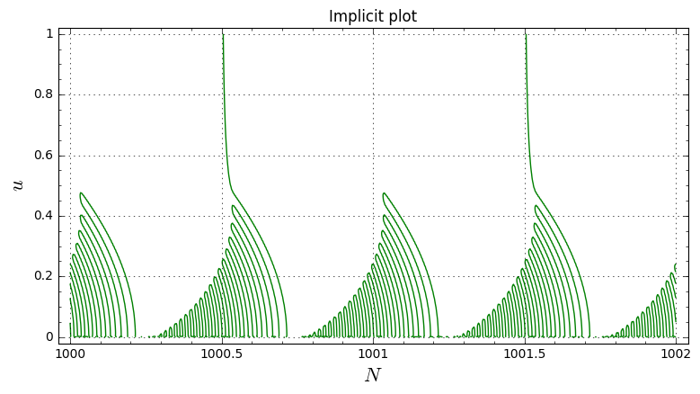
1. The peaks of the shark-fins on the whole numbered N's seem to almost precisely fill out the troughs of the shark-fins on the neighboring half numbered N's. So it seems there's some kind of sign based effect on the peaks alternating with a 1/2 N cadence.

Here are two neighboring shark-fins from P15's Zooming in on N[600, 602], u[0, 1] with 1000 summation terms plot overlaid:

2. The green shark-fin curves also kinda reminded me of oscilloscope plots for a generated signal trapped inside a shaped envelope. Suggesting that two distinct constraints may separately be generating the sweeps of these curves and the bounding (shark-fin shaped) envelopes.

3. The solid green apron shaped plots from P15's Second order Taylor expansion of final factor of log(n/N) in 1.18 appear much simpler, more regular, and half as tall as (a binary order of magnitude) the shark-fin shaped plots.

4. Looking at the peak_u values posted by P15, the product of (peak_u * sweep_count) seems to be relatively consistent, indicating that they may be scaling at some kind of inverse relationship relative to N:

N	peak_u	plot_author	sweep_count	peak_u * sweep_count
100	1.2734375	P15	12	15.28125
200	0.9609375	P15	18	17.296875
600	0.5859375	P15	32	18.75
1000	0.4609375	Rudolph	40	18.4375

Hypothesis:

I suspect that the interesting shark-fin and apron shaped plots may actually be surfacing artifacts of the precisions being used in the calculations. I would venture two guesses that:

a) the threshold value used by the zero finding algorithms (to determine how small a value needs to be to be considered a found zero) is responsible for the shark-fin/apron shape of the bounding envelopes

b) the precision being used for smaller values (represented using a form of binary floating-point numbers) within the calculations for the zeros in these interesting areas is responsible for introducing quantized errors (rounded up or down to the nearest whole binary fraction), and that that rounding causes the zero finding algorithms to detecting sweeping curves of zeros along the edges where the rounded values jump from rounding up or down to the nearest whole binary fractions.

Follow up questions:

1. Is there reason to be confident that the patterns in the interesting regions are not artifacts of the calculating implementations as I hypothesised?

2. Do P15's and Rudolph's implementations (arb vs pari/gp) produce the same number of sweeps in their shark-fin plots when evaluated at the same N? (e.g: N = 100, 200, 600, and 1000)

3. Does adjusting the threshold value used by the zero finding algorithms affect the shape, size, and/or position of the apparent bounding envelopes?

4. Can the sweeping curves of zeros within the shark-fin plots be affected/eliminated by using higher precision variables in the log(n/N) calculations?

Thoughts?

[p15-git-acc]

I suspect that the interesting shark-fin and apron shaped plots may actually be surfacing artifacts of the precisions being used in the calculations.

Thoughts?

Most of the numbers I've posted have been computed with interval arithmetic (not IEEE floating point) where I've checked the output interval, ruling out a large class of numerical artifacts. My plots have used only a single point evaluation per pixel so I suppose it's not impossible that the 'shark fins' are actually aliasing or moiré patterns, but I think it's really unlikely.

I find the suggestion that the 'shark fins' look kind of the Airy plot to be compelling.

[rudolph-git-acc]

@steffenyount

Thanks for sharing your thoughts and also for putting that famous scary 'Jaws'-theme in my head that I am humming now each time I look at these charts... :-)

The peaks of the shark-fins on the whole numbered N's seem to almost precisely fill out the troughs of the shark-fins on the neighboring half numbered N's. So it seems there's some kind of sign based effect on the peaks alternating with a 1/2 N cadence

I noticed something similar when counting the 'paired' real zero trajectories. It is peculiar that we end with a 'widowed' straight line at the half integers that can't find a 'buddy', where the whole integer 'fins' end with a pair. So, there is clearly something 'odd' and 'even' happening in these shark fins.

Can't of course fully rule out that the phenomenon observed originates from precision/accuracy issues, however do believe chances this is the case are low. We have used Arbitrary Precision software (ARB) for the initial plots that outlines the patterns (see the links in the OP of the eleventh Polymath15 thread) and did double checks agains pari/gp that yielded the same patterns.

I did do a quick count on the N[600, 602] plots from P15 and the one I produced in pari/gp and both have the same number of 'peaks' (15) in each fin (at the 1/2 and whole integers, not counting the straight lines).

[p15-git-acc]

Here's an example evaluation of (1.40) and (1.41) at the point x=1000, t=-10 (which has been used previously), and an interpretation of the results.

For (1.40) the sum is over n=1..1000 as was used in (1.20) previously. For (1.41) the sum is over m=-10..10 and the limits of the integral of (1.43) are X=[-100, 100] as suggested above.

Ht140: 2.571676382e-167 - 2.171715291e-167*i
Ht141: 2.655787101e-167 - 2.583308032e-167*i

The (1.40) output exactly matches the (1.20) output reported earlier in this thread, which is good because these are supposed to be identical. The (1.41) output is not wildly wrong, but it only matches one digit.

The difference between the (1.40) and (1.41) results could be due to any of several reasons. Maybe my code just has a typo, maybe the wiki has a typo, maybe I'm understanding the math wrong and (1.41) is only an approximation of (1.40) even with infinite summation and integral intervals, or maybe summation and/or integration truncation errors in one or both functions are responsible.

Realistically it might be that my code has a bug, but optimistically it's the truncation. Here are the results of increasing the summation limits to n=1..10000, m=-100..100 while keeping the same integration limits:

Ht140: 2.571676382e-167 - 2.171715291e-167*i
Ht141: 2.600887758e-167 - 2.425282241e-167*i

The (1.40) output remained unchanged, and the (1.41) output has slowly moved toward the (1.40) value.

My best guess is that my code is correct and that the suggested summation and/or integration limits for (1.41) and (1.43) do not apply for such small values of x and/or t, but I would be happy if someone could independently check these numbers in case my code is wrong.

[p15-git-acc]

Here's a comparison of (1.46) and (1.55) at the point x=1000, t=-10 and m=0. First I'll use the narrow integration limits [-10, 10] for (1.46):

g_0 (1.46): -0.2550392184 - 0.1657239403*i
g_0 (1.55): -0.2263597266 - 0.1471080986*i

They are quite different, so let's bump up the integration limits to [-100, 100]:

g_0 (1.46): -0.2540672147 - 0.1651145859*i
g_0 (1.55): -0.2263597266 - 0.1471080986*i

That brings (1.46) slightly closer to (1.55) but it's still off. How about [-1e8, 1e8]:

g_0 (1.46): -0.2540672147 - 0.1651145859*i
g_0 (1.55): -0.2263597266 - 0.1471080986*i

They are still different. I'm not sure what to make of this. Either I have a bug in my code, or the wiki has a typo, or somehow there is still a significant integration truncation error, or something is wrong mathematically with the shift of the contour of integration. Again independent confirmation of these numbers would be welcome!

[rudolph-git-acc]

P15: at x=1000, t=-10 I get in pari/gp the same result for 1.40:

n=1...1000 2.57167638200335132302999673776 E-167 - 2.17171529053235446607983959786 E-167*I

for 1.41 (with 1.42 the integral) I get for m=-10..10, X=N-100...N+100:

Ht141 -> Ht142: 5.34948647916775361632804266658 E-167 - 4.51458558239131276120704969076 E-167*I

for 1.41 (with 1.43 the integral) I get for m=-10..10, X=-100...+100:

Ht141 -> Ht143: 5.34948647916775361632804266658 E-167 - 4.51458558239131276120704969076 E-167*I

Tried changing m, X and the accuracy target/sampling points for the integral, but results are very unstable. Also tried higher x=100,000, t=-10,000 but results seems to be getting worse:

Ht120: 3.91291751919930940572842716616 E-16983 + 6.17150098907669030384569714344 E-16984*I
Ht140: 3.91291751919930940572842716616 E-16983 + 6.17150098907669030384569714344 E-16984*I
Ht141 -> Ht142: 1.29122865222068149698984496460 E-16982 - 1.27111357043491494779751829036 E-16982*I
Ht141 -> Ht143: 1.29122865222068149698984496460 E-16982 - 1.27111357043491494779751829036 E-16982*I 

It feels like the step from 1.40 to 1.41 still induces some noisy behaviour. 1.42 and 1.43 should be ok since they produce the same outcome. Since 1.43 'feeds' 1.46, could you share the values you get for 1.43?

Will now try Maple to see if things improve in another CAS.

[p15-git-acc]

Thanks Rudolph. To summarize, for x=1000, t=-10, m=-10..10, X=[-100, 100], sum=(1.41), integral=(1.43) you are getting 5.34948647916775361632804266658 E-167 - 4.51458558239131276120704969076 E-167*I whereas I am getting 2.655787101e-167 - 2.583308032e-167*i. With my library the integration subroutine gives rigorous bounds so I don't have to deal with accuracy target/sampling points, and for this integral in particular it reports convergence pretty quickly. It's still likely that I have some bug or typo in my code. If you have pari/gp code could you paste/submit it so I could check numerical values of sub-expressions to detect typos in my code?

Since 1.43 'feeds' 1.46, could you share the values you get for 1.43?

The only difference between 1.43 and 1.46 is the renaming of the expressions a, b, c, right? I have to do that kind of thing anyway in my code, so there is no difference to how I would implement them.

[rudolph-git-acc]

Sure, here is the code (please note the parameter setting at the end of the integral (number of 2^sampling points) that proved to be quite sensitive).

EDIT 1: added M0.

EDIT 2: fixed the fractional parts I had missed

M0(s)=return(s*(s-1)/2*Pi^(-s/2)*sqrt(2*Pi)*exp((s/2-1/2)*(log(s/2))-s/2));

Ht140(x,t) = {
    xt = x-Pi*abs(t)/4;
    N = sqrt(xt/(4*Pi));
    u = 4*Pi*abs(t)/xt;
    mulfact = exp(Pi^2*t/64)*(M0((1+I*xt)/2))*N^(-(1+I*xt)/2)/(8*sqrt(1-I*u/(8*Pi)))*exp(3*Pi*I*N^2);
    A=mulfact*sum(n=1,1000,exp(-u*(n-N)^2/(4*(1-I*u/(8*Pi)))-2*Pi*I*n*frac(2*N+1/2)-2*Pi*I/(3*N)*(n-N)^3));
    return(A);
}

Ht1412(x,t) = {
    xt = x-Pi*abs(t)/4;
    N = sqrt(xt/(4*Pi));
    u = 4*Pi*abs(t)/xt;
    mulfact = exp(Pi^2*t/64)*(M0((1+I*xt)/2))*N^(-(1+I*xt)/2)/(8*sqrt(1-I*u/(8*Pi)))*exp(3*Pi*I*N^2);
    A=mulfact*sum(m=-10,10, Ht142(N, u, m));
    return(A);
}

Ht1413(x,t) = {
    xt = x-Pi*abs(t)/4;
    N = sqrt(xt/(4*Pi));
    u = 4*Pi*abs(t)/xt;
    mulfact = exp(Pi^2*t/64)*(M0((1+I*xt)/2))*N^(-(1+I*xt)/2)/(8*sqrt(1-I*u/(8*Pi)))*exp(3*Pi*I*N^2);
    A=mulfact*sum(m=-10,10, Ht143(N, u, m));
    return(A);
}

Ht142(N, u, m) = {
    A=intnum(X=N-100,N+100,exp(-u*((X-N)^2)/(4*(1-I*u/(8*Pi)))+2*Pi*I*X*(m-frac(2*N+1/2))-2*Pi*I/(3*N)*(X-N)^3),5);
    return(A);
}

Ht143(N, u, m) = {
    A=exp(2*Pi*I*N*(m-frac(2*N+1/2)))*intnum(X=-100,100,exp(-u*(X^2)/(4*(1-I*u/(8*Pi)))+2*Pi*I*(X)*(m-frac(2*N+1/2))-2*Pi*I/(3*N)*X^3),5);
    return(A);
}

print("Ht140: ", Ht140(1000, -10));
print("Ht141 -> Ht142: ", Ht1412(1000, -10));
print("Ht141 -> Ht143: ", Ht1413(1000, -10));

[p15-git-acc]

I already see expressions like (m-(2*N+1/2)) in that pari/gp code. On the wiki it's written as (m - {2*N + 1/2}) with the notation that {x} is the fractional part of x.

[rudolph-git-acc]

Great catch. Had missed that indeed !

EDIT: have fixed it in code above.

[p15-git-acc]

M0 in the pari/gp code is missing the 1/8 that's in the writeup. I'm not sure if that's deliberate. My guess is that you had been using M0 as a factor of an expression that was normalised by dividing by its absolute value so the real factors of M0 cancelled and it didn't matter.

Edit: I see the 1/8 is just moved out of M0 and into a different part of the multiplier

[teorth]

Thanks for all the numerics!

Regarding the discrepancy between (1.43) and (1.55): if one could also compute the intermediate expressions (1.46), (1.50), (1.55) (and perhaps also (1.52), (1.53), (1.54) for the value of x indicated by (1.55)) this should localise the error.

As for the discrepancy between (1.40) and (1.41): this is a bit disturbing, but may be due to the low values of x and t. Ideally we should take a test point (x,t) from the same region that our (N,u) plot is coming from, e.g. take N=1000, u=0.4 and then solve for t = -uN^2, x = 4 Pi N^2 + Pi t / 4 [EDIT: I meant x = 4 Pi N^2 - Pi t / 4]. The Poisson summation formula is in principle exact so what must be happening is either the m summation is decaying too slowly or the X integral is decaying too slowly. One possibility is that the X cutoff of the oscillatory integral is creating some unwanted oscillation; it could be that simply increasing the range of integration of X will solve this isue.

[rudolph-git-acc]

Yes! Substantially increasing x and -t as you suggested perfectly aligns 1.40 with 1.41 (and 1.42 + 1.43). This is at m=-10..10 and X = -100...+100:

print("Ht140: ", Ht140(10000000, -400000));
print("Ht141 -> Ht142: ", Ht1412(10000000, -400000));
print("Ht141 -> Ht143: ", Ht1413(10000000, -400000));

Ht140: -8.58800587195526020181918485414 E-1678676 + 5.54164658493373478236289025249 E-1678677*I
Ht141 -> Ht142: -8.58800587195526020181918485414 E-1678676 + 5.54164658493373478236289025249 E-1678677*I
Ht141 -> Ht143: -8.58800587195526020390526458953 E-1678676 + 5.54164658493373475201667687004 E-1678677*I

Tested other values and get very stable results. Even t=-400 still gives good results at this height of x.

[rudolph-git-acc]

Have tested up to 1.50 and all results look fine. I only had to increase accuracy of the integral when moving from 1.46 to 1.50. All other sum an integral limits (m, XYZ) remained the same.

Still struggling with 1.51 and wondered whether the 4*I*b^3*a^(-2)/3 should be 2*I*b^3*a^(-2)/3 ?

[p15-git-acc]

Still struggling with 1.51 and wondered whether the 4*I*b^3*a^(-2)/3 should be 2*I*b^3*a^(-2)/3 ?

This change works for me. For N=1000, u=2/5, m=0 (1.55) now numerically matches (1.46) and (1.50). I'm certain this is a typo on the wiki.

[p15-git-acc]

Here are four pictures of roots (observed sign change, or computed interval at a point includes zero) of (1.41, 1.55) with N=[1000, 1002], u=[0, 1], after making Rudolph's correction:

m=-10..10:

m=-1..1:

m=0..1:

m=0:

From the pictures it's clear that you only need the first two terms of the sum, as had been speculated. This means that the complex behavior can be captured with a smallish closed form expression, if you care about that kind of thing and if you count the airy function as closed form. You could write it on a napkin without drawing the summation or integral symbols.

[rudolph-git-acc]

Amazing! Just out of curiosity, does your last plot have the same x-axis scale as the others? I.e. do the lines at m=0 exactly separate a pair of two 'fins' ?

ADDED: and if your napkin is really small, how about using this approximation for the Airy-function and maybe cancel a few terms :

EDIT: that unfortunately doesn't work, since it is only valid for r > 0.

[p15-git-acc]

does your last plot have the same x-axis scale as the others?

Yes all four plots are on the same scale. Sorry I don't have axes labeled, I am constructing the image pixel-by-pixel instead of using a proper plotting package.

By the way, I checked the m=0 approximation at three points, and it looks like the real part is negative on the outside of those two lines and positive between them, so those lines do represent actual changes in the sign of the real part. The imaginary part is non-negligible.

On the wiki I'm not sure what is meant by "we could hope to use one of the known asymptotics of the Airy function to get a more tractable approximation"; it's already very numerically tractable for me thanks to the weirdly over-engineered Airy implementation in the library I'm using. Perhaps the hope is to apply an asymptotic approximation of Airy that is easier to break apart and manipulate and gives more insight into the behavior of the zeros, rather than simply speeding up the evaluation.

[teorth]

Great! This is a lot of progress. I've corrected the typo on the wiki and wrote down the "napkin" approximation as (1.56) (hopefully there are no typos).

p15: yes, I am hoping to use a suitable asymptotics of the Airy function to make this napkin approximation even more theoretically tractable, in particular to explain the asymmetric oscillations, the sharkfin shape, and the somewhat strange power law we saw between u and N. It's great though that it's so numerically tractable - for instance one could now try exploring much larger values of N and u which should at least clarify the power law.

I'll try to work out these asymptotics tomorrow - as Rudolph points out, the Airy function is a bit weird in that it has different asymptotics in different directions in the complex plane. But I think we're almost there now - I'm very happy to see that all the sums and integrals are gone!

EDIT: we may as well just try our luck and plug in the approximation Ai(r) ~ 1/(2 sqrt(Pi)) r^(-1/4) exp( - 2/3 r^(3/2) ) even though we will be using a complex argument. Hopefully we get something vaguely resembling the sharkfin plot!

[p15-git-acc]

That asymptotic approximation works well enough numerically, even for a complex argument.

For N=1000, u=0.4, m=0:

g155_0: 1.138314675e-08 + 2.413676122e-09*i
g155_approx_0: 1.139225816e-08 + 2.415456591e-09*i

For N=[1000,1002], u=[0,1], m={0,1}:

[teorth]

Wow, that does look promising!

I've substituted the Airy approximation on the wiki to obtain a messy but explicit approximation to H_t as (1.58). If one could double check that this is still giving the sharkfin plot for the zeroes this would be great. Also it is not obvious to me why this approximation should be approximately real; would it be possible to test it at a few values to see how small the imaginary part is compared with the real part?

It is tempting just to set this equation to zero (not just the real part) and start solving for it. The thing though is that without an explanation for why this expression should be real valued, one should get very few exact zeroes (if one wants to set the real and imaginary parts simultaneously equal to zero then in the (N,u) plane one should just get some isolated points as zeroes, not curves). So there is still a bit of mystery. On the other hand, the approximation we have now is completely in terms of elementary functions, without any sums or integrals, and so it should be possible to compute all the asymptotics by direct calculation (maybe with a few more Taylor expansions to try to clean things up a bit more).

[p15-git-acc]

Here's a table that shows the decay of the height of the shark fin centered at N. It's rough because I just made upside down images 2000 pixels tall and wrote down the pixel coordinate that I found with my mouse in an image viewer. It uses the asymptotic approximation of Ai.

N	u*1000
30	1923
100	1285
300	820
1000	481
3000	289
10000	163
30000	96
100000	54
300000	32
1000000	18

[p15-git-acc]

Also it is not obvious to me why this approximation should be approximately real

First I'll back up to the true Airy function and show the usual plot N=[1000, 1002], u=[0, 1], m={0, 1}, but this time with the zeros of the imaginary part (red) as well as the zeros of the real part (green):

Zooming in on the fin centered at N=1000:

And finally, switching to the asymptotic Airy approximation:

Although the last two pictures look similar, the one made with the true Airy formula has zeros of the real and complex parts approaching each other as u approaches zero whereas the one made with the asymptotic Airy approximation has zeros of the real and complex parts interlacing each other as u approaches zero.

[rudolph-git-acc]

Working on 1.58 and could there be a small typo in the brackets in the exp in final part (i.e. the bracket should move from behind a^4/3 to behind 2pi a^-1/3 ?

[p15-git-acc]

Here's a more colorful (but probably less informative) rendering of the asymptotic Airy approximation fin plot above, using color scheme 4 from here: A multiplier has been normalized for this plot.

[rudolph-git-acc]

Sharkfins have never looked better, P15 :)

Here is the plot for 1.58 (also had to use M/|M| as the normalised multiplier). I do however pick up a few more straight lines. Haven't yet figured out where these come from:

Code used:

Ht158(N, u, m) = {
    a=2*Pi/N;
    b=I*u/(4*(1-I*u/(8*Pi)));
    c0=2*Pi*(0-frac(2*N+1/2));
    mulfact = exp(Pi^2*(-u*N^2)/64)*(M0((1+I*(4*Pi*N^2))/2))*N^(-(1+I*(4*Pi*N^2))/2)/(8*sqrt(1-I*u/(8*Pi)))*exp(3*Pi*I*N^2)*2*Pi*a^(-1/3)*exp(I*N*c0+2/3*I*b^3*a^(-2)+I*b*c0/a);
    A1=-(c0*a^(-1/3)+b^2*a^(-4/3))^(-1/4)*exp(-2/3*(-(c0*a^(-1/3)+b^2*a^(-4/3)))^(3/2));
    A2=exp(2*Pi*I*N +2*Pi*I*b/a)*(-(c0*a^(-1/3)+b^2*a^(-4/3)+2*Pi*a^(-2/3)))^(-1/4)*exp(-2/3*(-(c0*a^(-1/3)+b^2*a^(-4/3)+2*Pi*a^(-1/3)))^(3/2));
    A=1/(2*sqrt(Pi))*mulfact*(A1+A2);
    return(A);
}

ADDED: getting the same picture for the imaginary parts:

[p15-git-acc]

That picture is different than the one I made in enough ways that I think there is a difference in the formulas we used. Your picture is nicer looking so I probably have a typo in my approximation code.