Help need for evaluation of latest wiki page equations

[rudolph-git-acc]

Grateful for any help to properly evaluate the sequence of equations on this Wiki page: http://michaelnielsen.org/polymath1/index.php?title=Polymath15_test_problem#Large_negative_values_of_.5Bmath.5Dt.5B.2Fmath.5D

Below is the pari/gp code I have used so far. At the end of the code is a simple rootfinder that should (approximately) find this sequence of roots:

-10.00000000, 906.72649548
-10.00000000, 931.47009390
-10.00000000, 976.80075639
-10.00000000, 990.45190417

however from eq 318 onwards it finds many more roots (also at different t, e.g. -100). Have experimented with the integral limits, the integral's fixed parameter, the real precision settings of pari and the size of the sums, but no success yet.

Have re-injected some of the non-zero multiplication factors that can be switched on/off if needed.

One thing I noticed is that after eq 307 the function doesn't seem to be real anymore (see data at the end). Not sure if this should matter though, since I use the real value of Ht for root finding.

default(realprecision, 40)

Xi(s)=return((s/2)*(s-1)*Pi^(-s/2)*gamma(s/2)*zeta(s));
M0(s)=return(s*(s-1)/2*Pi^(-s/2)*sqrt(2*Pi)*exp((s/2-1/2)*log(s/2)-s/2));

Ht302(x,t) = {
    A=intnum(v=-8,8,Xi((1+I*x)/2+I*sqrt(abs(t))*v)*exp(-v^2),1);
    return(A);
}

Ht303(x,t) = {
    A=intnum(v=-8,8,Xi((1+I*x)/2+I*sqrt(abs(t))*v-Pi*I*abs(t)/8)*exp(-(v-Pi*sqrt(abs(t))/8)^2),1);
    return(A);
}

Ht304(x,t) = {
    xt = x-Pi*abs(t)/4;
    mulfact = exp(-Pi^2*abs(t)/64);
    A=mulfact*intnum(v=-8,8,Xi((1+I*xt)/2+I*sqrt(abs(t))*v)*exp(-v^2+Pi*sqrt(abs(t))*v/4),1);
    return(A);
}

Ht307(x,t) = {
    xt = x-Pi*abs(t)/4;
    mulfact = exp(-Pi^2*abs(t)/64)*2;
    A=mulfact*intnum(v=-8,8,real(M0((1+I*xt)/2+I*sqrt(abs(t))*v))*zeta((1+I*xt)/2+I*sqrt(abs(t))*v)*exp(-v^2+Pi*sqrt(abs(t))*v/4),1);
    return(A);
}

Ht312(x,t) = {
    xt = x-Pi*abs(t)/4;
    mulfact = exp(-Pi^2*abs(t)/64)*(M0((1+I*xt)/2));
    A= mulfact*intnum(v=-8,8,exp((I*sqrt(abs(t))*v)/2*log(xt/(4*Pi))-Pi*sqrt(abs(t))*v/4+(I*abs(t)*v^2)/(2*xt))*zeta((1+I*xt)/2+I*sqrt(abs(t))*v)*exp(-v^2+Pi*sqrt(abs(t))*v/4),1);
    return(A);
}

Ht315(x,t) = {
    xt = x-Pi*abs(t)/4;
    N = sqrt(xt/(4*Pi));
    u = 4*Pi*abs(t)/xt;
    mulfact = exp(-Pi^2*abs(t)/64)*(M0((1+I*xt)/2));
    A=mulfact*intnum(v=-8,8,exp(I*sqrt(abs(t))*v*log(N)+I*u*v^2/(8*Pi))*zeta((1+I*xt)/2+I*sqrt(abs(t))*v)*exp(-v^2),1);
    return(A);
}

Ht316(x,t) = {
    xt = x-Pi*abs(t)/4;
    N = sqrt(xt/(4*Pi));
    u = 4*Pi*abs(t)/xt;
    mulfact = exp(-Pi^2*abs(t)/64)*(M0((1+I*xt)/2));
    A=mulfact*sum(n=1,1000, intnum(v=-8,8,exp(I*sqrt(abs(t))*v*log(N)+I*u*v^2/(8*Pi))*n^(-((1+I*xt)/2+I*sqrt(abs(t))*v))*exp(-v^2),1));
    return(A);
}

Ht317(x,t) = {
    xt = x-Pi*abs(t)/4;
    N = sqrt(xt/(4*Pi));
    u = 4*Pi*abs(t)/xt;
    mulfact = exp(-Pi^2*abs(t)/64)*(M0((1+I*xt)/2))*N^((1+I*xt)/2)/8;
    A=mulfact*sum(n=1,1000, intnum(v=-8,8,exp(-I*sqrt(abs(t))*v*log(n/N)+I*u*v^2/(8*Pi)-((1+I*xt)/2)*log(n/N))*exp(-v^2),1));
    return(A);
}

Ht318(x,t) = {
    xt = x-Pi*abs(t)/4;
    N = sqrt(xt/(4*Pi));
    u = 4*Pi*abs(t)/xt;
    mulfact = exp(-Pi^2*abs(t)/64)*(M0((1+I*xt)/2))*N^((1+I*xt)/2)/8*sqrt(Pi);
    A=mulfact*sum(n=1,1000,exp(-abs(t)*(log(n/N))^2/(4*(1-I*u/(8*Pi)))-(1+I*xt)/2*log(n/N)));
    return(A);
}

Ht320(x,t) = {
    xt = x-Pi*abs(t)/4;
    N = sqrt(xt/(4*Pi));
    u = 4*Pi*abs(t)/xt;
    mulfact = exp(-Pi^2*abs(t)/64)*(M0((1+I*xt)/2))*N^((1+I*xt)/2)/8*sqrt(Pi);
    A = mulfact*sum(n=1,1000,exp(-(abs(t)*(n-N)^2)/(4*N^2*(1-I*u/(8*Pi)))-I*xt/2*(n-N)/N+I*xt*(n-N)^2/(4*N^2)));
    return(A);
}

Ht321(x,t) = {
    xt = x-Pi*abs(t)/4;
    N = sqrt(xt/(4*Pi));
    u = 4*Pi*abs(t)/xt;
    mulfact = exp(-Pi^2*abs(t)/64)*(M0((1+I*xt)/2))*N^((1+I*xt)/2)/8*sqrt(Pi);
    A = mulfact*sum(n=1,1000,exp(-(2*Pi*u*(n-N)^2)/(8*Pi-I*u)-2*Pi*I*N*(n-N)+Pi*I*(n-N)^2));
    return(A);
}

Ht323(x,t) = {
    xt = x-Pi*abs(t)/4;
    N = sqrt(xt/(4*Pi));
    u = 4*Pi*abs(t)/xt;
    mulfact = exp(-Pi^2*abs(t)/64)*(M0((1+I*xt)/2))*N^((1+I*xt)/2)/8*sqrt(Pi);
    A = mulfact*sum(n=1,1000,exp(-(2*Pi*u*(n-N)^2)/(8*Pi-I*u)-Pi*I*n^2+2*Pi*I*(n-N)^2));
    return(A);
}

Ht324(x,t) = {
    xt = x-Pi*abs(t)/4;
    N = sqrt(xt/(4*Pi));
    u = 4*Pi*abs(t)/xt;
    mulfact = exp(-Pi^2*abs(t)/64)*(M0((1+I*xt)/2))*N^((1+I*xt)/2)/8*sqrt(Pi);
    A = mulfact*sum(n=1,1000,exp((16*Pi^2*I*(n-N)^2)/(8*Pi-I*u))*exp(Pi*I*n));
    return(A);
}

Ht328(x,t) = {
    xt = x-Pi*abs(t)/4;
    N = sqrt(xt/(4*Pi));
    u = 4*Pi*abs(t)/xt;
    mulfact = exp(-Pi^2*abs(t)/64)*(M0((1+I*xt)/2))*N^((1+I*xt)/2)/8*sqrt(Pi);
    A = mulfact*sum(n=1,1000,exp(-Pi*I*n*(n+1)/2)*exp(2*Pi*I*(n+1/2)*N)*exp(-u*n*(n+1)/16));
    return(A);
}

print("eq.302 ",Ht302(1000, -10))
print("eq.303 ",Ht303(1000, -10))
print("eq.304 ",Ht304(1000, -10))
print("eq.307 ",Ht307(1000, -10))
print("eq.315 ",Ht315(1000, -10))
print("eq.316 ",Ht316(1000, -10))
print("eq.317 ",Ht317(1000, -10))
print("eq.318 ",Ht318(1000, -10))
print("eq.320 ",Ht320(1000, -10))
print("eq.321 ",Ht321(1000, -10))
print("eq.323 ",Ht323(1000, -10))
print("eq.324 ",Ht324(1000, -10))
print("eq.328 ",Ht324(1000, -10))

xs = 900; xe = 1010;
ts = -10; te = -1;
f=Ht318;
forstep(t=ts, te, 10, {
    xc = xs;
    while(xc <= xe,
        if(real(f(xc,t))*real(f(xc+1,t)) < 0, root=solve(a=xc, xc+1, real(f(a,t))); printf("%3.8f, %3.8f\n",t, root));
        xc=xc+1);
})

eq.302 1.201485926838305713580758240853488704456 E-165 + 3.514303326279329051 E-221*I
eq.303 1.201485926838305713582303927841938470920 E-165 + 3.522103826014908131 E-221*I
eq.304 1.201485926838305713582303927841938470920 E-165 + 3.522103826014922598 E-221*I
eq.307 1.201477416607903787215861199656638682224 E-165 + 3.992587328505261451855248837227037420869 E-169*I
eq.312 1.200242494404236645648308584282451391036 E-165 + 4.014384445003979486997306873566995218158 E-169*I
eq.315 1.200242494404236645648308584282451391036 E-165 + 4.014384445003979486997306873566995218158 E-169*I
eq.316 1.200242494404236645648308630967087228353 E-165 + 4.014384445003979487000178658198142256762 E-169*I
eq.317 1.210630457223022714918883693478442584040 E-165 - 5.581422172204223838770738013241198104262 E-166*I
eq.318 1.209227903617935860382758702133562335051 E-165 - 5.611945144292097211229689587084475461023 E-166*I
eq.320 2.791674127351571571455964690537038072397 E-167 - 2.126109533152847673586778474944806978351 E-167*I
eq.321 2.791674127351571571455964690537038072397 E-167 - 2.126109533152847673586778474944806978351 E-167*I
eq.323 -3.076893561828845392623560432368639943370 E-167 + 1.687160985046708488717820653125387727510 E-167*I
eq.324 -3.076893561828845392623560432368639943370 E-167 + 1.687160985046708488717820653125387727510 E-167*I
eq.328 -3.076893561828845392623560432368639943370 E-167 + 1.687160985046708488717820653125387727510 E-167*I

[p15-git-acc]

Analysing the new decay table I get u^(2.18535) ~ (173.284)/N.

[p15-git-acc]

In the comment above, should "x = 4 Pi N^2 + Pi t / 4" be changed to "x = 4 Pi N^2 - Pi t / 4" or "x = 4 Pi N^2 + Pi abs(t) / 4"?

[teorth]

Rudolph, p15: thanks for the typos.

It seems that the asymptotic formula for Airy is introducing some phase drift (as the real and imaginary zeroes are decohered from each other), but it is interesting that nevertheless the real zeroes are producing a visually identical plot to earlier, more accurate, approximations. This bodes well regarding the robustness of the phenomenon, we can probably get away with moderately sloppy approximations at this point and still hope to get a very similar plot.

The extra vertical lines are likely artefacts from the coordinate singularity formed by the introduction of the {2N+1/2} fractional part. Fortunately this singularity is like the international date line - it doesn't seem to cut across anything important :)

I'm guessing that in the region of interest, the b^2 a^{-4/3} terms are significantly larger than the c_0 a^{-1/3} and 2 pi a^{-1/3} terms, suggesting that a Taylor expansion around b^2 a^{-4/3} may lead to a further approximation of (1.58) by something simpler that would still give a visually similar plot for the zeroes of the real part. Hopefully I'll have some time later this evening to actually compute this.

[p15-git-acc]

I now think the Ht158 pari/gp code has something wrong with it.

Here are three examples where I evaluate N=1000, u=0.4, m={0,1}:

Ht_141_146: -5.885034858e-2169946 + 1.045353076e-2169946*i
Ht_141_155: -5.885034858e-2169946 + 1.045353076e-2169946*i
Ht_141_155_approx: -5.8897215e-2169946 + 1.046262651e-2169946*i

Here are two more, from the pari/gp code:

Ht1413: -5.8850348581225816301452269816410068510 E-2169946 + 1.0453530764660909945676594598962344252 E-2169946*I
Ht158: 4.9045176790638947260288688132054130807 E-2169946 + 3.4248396250406610127560276858661910599 E-2169946*I

[teorth]

This may be premature if there are numerical issues with 1.58, but I attempted a preliminary Taylor approximation to 1.58 on the wiki, ending up at 1.65. However I am a bit dubious as to exactly how accurate this is going to be (but hopefully one of the intermediate steps between 1.58 and 1.65 remains accurate, or at least gives something visually similar to the sharkfin shape, and we can continue on from there).

[p15-git-acc]

I looked at (1.58) and its pari/gp implementation some more.

There is one typo in (1.58) on the wiki. At the very end of the (1.58) line, e^-2/3(-(...)^{3/2}) should be re-parenthesized to e^-2/3(-(...))^{3/2}.

This typo was implicitly fixed in the pari/gp code, but the code had two typos that weren't on the wiki. The first was a similar parenthesis issue at the beginning of its definition of A1 where -(...)^(-1/4) should be changed to (-(...))^(-1/4). The second was that the code had an a^(-2/3) that should be a^(-1/3). I've rewritten the pari/gp function below with these changes, and I've also removed the unused argument m.

Ht158(N, u) = {
    a=2*Pi/N;
    b=I*u/(4*(1-I*u/(8*Pi)));
    c0=2*Pi*(0-frac(2*N+1/2));
    mulfact = exp(Pi^2*(-u*N^2)/64)*(M0((1+I*(4*Pi*N^2))/2))*N^(-(1+I*(4*Pi*N^2))/2)/(8*sqrt(1-I*u/(8*Pi)))*exp(3*Pi*I*N^2)*2*Pi*a^(-1/3)*exp(I*N*c0+2/3*I*b^3*a^(-2)+I*b*c0/a);
    A1=(-(c0*a^(-1/3)+b^2*a^(-4/3)))^(-1/4)*exp(-2/3*(-(c0*a^(-1/3)+b^2*a^(-4/3)))^(3/2));
    A2=exp(2*Pi*I*N +2*Pi*I*b/a)*(-(c0*a^(-1/3)+b^2*a^(-4/3)+2*Pi*a^(-1/3)))^(-1/4)*exp(-2/3*(-(c0*a^(-1/3)+b^2*a^(-4/3)+2*Pi*a^(-1/3)))^(3/2));
    A=1/(2*sqrt(Pi))*mulfact*(A1+A2);
    return(A);
}

[teorth]

I think I fixed the missing parenthesis on the wiki (by the way feel free to edit the wiki directly for typos like this).

[p15-git-acc]

I think the last -3/2 in the (1.61) identity should be 3/2, and (1.62) and (1.63) are way off numerically for me so maybe this typo has propagated.

[rudolph-git-acc]

Thanks for catching these typo's P15! The "international data lines" have now also vanished :)

[p15-git-acc]

The real part of b is actually smaller than a for the test point N=1000, u=2/5 and abs(a*c0 / b^2) is about 2. This means that the (1.62) expansion won't work for that test point even if the formula has an error and if the error is fixed.

[p15-git-acc]

From (1.61) to (1.62) it looks like -(2/3)(-b^2 a^(-4/3))^(3/2) is being simplified to (2 i b^3)/(3 a^2) which I think isn't valid for our values of a and b.

[teorth]

Hmm, OK, I fixed some typos but I think based on what you say I'm prepared to abandon the calculations in (1.59)-(1.64) and think of another approximation. I guess the presence of the N in the denominator in a isn't as dominating as I thought it would be...

One possible thing to look for is any change in behaviour in the arguments - (c_0 a^{-1/3} + b^2 a^{-4/3} ) ) and - (c_0 a^{-1/3} + b^2 a^{-4/3} + 2\pi a^{-1/3}) ) near the boundary of the sharkfin. For instance does the phase or magnitude of these complex numbers do anything unusual near the boundary?

EDIT: after fixing all the sign errors, I end up with an approximation that vanishes when N is a half-integer, i.e. I just get the vertical lines. Basically I think the approximation (1.64) is only good when u is large (so b is not too small and so a*c0/b^2 is not huge).

[p15-git-acc]

I'm getting (1.64) a few thousand orders of magnitude off numerically, so something is still wrong with it or I made a mistake copying it from the wiki.

Ht164(N, u) = {
        t = -u*N*N;
        x = 4*Pi*N*N - Pi*t/4;
        xt = x-Pi*abs(t)/4;
        a=2*Pi/N;
        b=(I*u)/(4*(1-(I*u)/(8*Pi)));
        c0=2*Pi*(0-frac(2*N+1/2));
        Ma=exp(Pi*Pi*t/64)/sqrt(1-(I*u)/(8*Pi));
        Mb=M0((1+I*xt)/2);
        Mc=N^(-(1+I*xt)/2);
        Md=exp(3*Pi*I*N*N)*2*Pi*a^(-1/3);
        Me=exp(I*N*c0+2*I*b*b*b/(3*a*a)+I*b*c0/a);
        mulfact=(1/8)*Ma*Mb*Mc*Md*Me;
        A1=(1/(2*sqrt(Pi)))*mulfact*(-b*b*(a^(-4/3)))^(-1/4);
        A2=-(a*c0)/(4*b*b) - (2*I*b*b*b)/(3*a*a) - (I*c0)/(a*b) - (I*c0*c0)/(4*b);
        A3=1+exp(2*Pi*I*N-Pi*I*(c0+Pi)/b);
        A=A1*exp(A2)*A3;
        return(A);
}

Also I think the expansion in (1.62) should be like 1 + (3/2)x + (3/8)x^2 instead of like 1 + (3/2)x + (1/8)x^2, but I don't think this typo propagates.

[p15-git-acc]

For instance does the phase or magnitude of these complex numbers do anything unusual near the boundary?

Here are the domain coloring plots of these two functions on N=[1000, 1002], u=[0, 1], normalized by the magnitude at N=1001, u=2/5. In this coloring scheme the phase is rendered as hue and the magnitude is rendered as brightness. Red is positive real, and cyan is negative real.

with c0:

with c1:

[p15-git-acc]

Here's another rendering of the second function above, ignoring magnitude. Positive reals are white, negative reals are black, complex numbers in the upper half plane are orange/gold, and complex numbers in the lower half plane are blue.

[teorth]

Thanks for the plots! They were less revealing than I had hoped, though - nothing interesting seems be happening at the boundary of the sharkfin region.

I'm running out of ideas now... maybe a plot of the ratio between the two summands in (1.58) will reveal something. For instance the zeroes of (1.58) - the places where the green and red curves cross - are the places where this ratio is equal to -1, so I feel like this ratio should at least "feel" the left edge of the sharkfin. (If it is possible to superimpose these sorts of plots with one of the sharkfin plots that might also give some clues.) There is some cancellation in the ratio that might make it easier to analyse than each of the individual summands (in particular, it's tempting to use the difference of two squares formula $x^{3/2} - y^{3/2} = \frac{x^3-y^3}{x^{3/2} + y^{3/2}}$ for the exponent...)

I fixed the typo you pointed out in (1.62) but I think I am willing to concede that (1.64) is basically unsalvageable for small u (might be accurate for large u though).

[rudolph-git-acc]

P15: tried your pari/gp code for 1.64 and the strange thing is that A3 always comes out as 2 whatever (N, u) one picks when N is an integer. The reason is that c0 is then always equal to -Pi hence the second part of A3 is always zero. Checked it against the Wiki and the code looks fine. So, the issue seems to be that A3 doesn't do anything in 1.64 for N = integer. Tried some fractional parts for N and the results can then be shifted up/down (EDIT: this probably shouldn't matter for the plots where we feed it with non-integer N).

[p15-git-acc]

Thanks for checking it!

[p15-git-acc]

a plot of the ratio between the two summands in (1.58)

Here's a domain coloring plot of the ratio of the second summand to the first summand. It uses the default color scheme where phase is rendered as hue and the magnitude is rendered as brightness.

If it is possible to superimpose these sorts of plots with one of the sharkfin plots

Here's the plot of roots of the real part of (1.58):

And superimposing the two images using a command like $ convert file1.png file2.png -background white compose darken -flatten file3.png:

[p15-git-acc]

The green shark-fin curves also kinda reminded me of oscilloscope plots for a generated signal trapped inside a shaped envelope

Here I've superimposed the plot of roots of the real part of (1.58) in green and the plot of roots of the difference of the magnitudes of the summands of (1.58) in red. As usual we have N=[1000, 1002], u=[0, 1].

[teorth]

Okay! So it looks like the magnitude of the ratio is determining the left edge of the sharkfin, and the phase of the ratio is determining the oscillations, with the right edge of the sharkfin being where the phase stops oscillating. It shouldn't be too hard to find simpler forms for these two expressions; this should finally give us a compact description of the sharkfin shape and size, at which point I think we can declare victory (there is of course the issue of making all of these dodgy asymptotics rigorous, but this can perhaps be a project for the future - for instance I have a graduate student in this area who might be interested in formalising these observations).

I should have some time later today to do the relevant computations.

UPDATE: I've written the ratio as an exponential exp(S) of a (slightly multivalued) quantity S defined in (1.65) on the wiki. The real part of S, representing the magnitude of the ratio, is unambiguous and is given in (1.66). So the zeroes of this quantity (or at least the level sets) should pick up the left edge of the sharkfin hopefully, going by p15's plots. This function is still a bit messy, but is becoming more and more elementary and hopefully it will become clear soon exactly what that left edge is at least. Then one has to understand why the imaginary part of S suddenly stops changing at the right edge of the sharkfin, and we'll have a pretty good qualitative understanding of this pattern soon!

[p15-git-acc]

I got as far as finding N*Re[i*b] = -N*u/(4*(1 + (u/(8*pi))^2)).

[rudolph-git-acc]

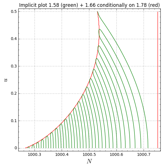
Here is a plot of 1.66 superimposed on 1.58:

Struggling a bit with the mod(Pi*I/2) in 1.65. How could that best be evaluated?

[p15-git-acc]

The real part of S (representing the magnitude of the ratios)

Should this say the logarithm of the magnitude of the ratios on the wiki? Although I guess it does technically represent the magnitude, by way of its logarithm.

[teorth]

OK, so it looks like we've identified the left edge of the sharkfin as the zero curve of (1.66). That's progress!

As for the modulus, this is mostly coming from the multivalued nature of the complex logarithm. One could simply use the standard branch of the logarithm and drop the mod pi i/2 altogether, and hopefully the imaginary part of (1.65) will then notice the right edge of the sharkfin which to me is the remaining unexplained feature. From p15's colour plots it looks like Im(S) is rapidly changing inside the sharkfin but somehow stops doing so once one exits the right edge of the sharkfin.

One may eventually study a derivative of Im(S) (with respect to, say, N) rather than Im(S) itself, as this is unambiguous (no need to mess around with branch cuts, since d/dz log(z) = 1/z has no branches).

p15: yes, I meant log of the magnitude. In particular, for the ratio to be of magnitude 1, the real part of S should vanish, which helps explain why the Re(S)=0 curve in Rudolph's plots are picking up the left edge of the sharkfin.

[p15-git-acc]

the right edge of the sharkfin which to me is the remaining unexplained feature

Near the right edge of the sharkfin, the argument -(c_0 a^{-1/3} + b^2 a^{-4/3} + 2\pi a^{-1/3}) ) rotates from negative real to positive real through the upper half plane, according to the rendering above, but this isn't a full explanation.

[rudolph-git-acc]

Closing in on the right edge of the shark fin, however not entirely there. I noted that the imaginary part of 1.65 stays around 6300i and moves only a small bit when changing N, u. The first term 2PiI*N in 1.65 seems to be responsible for this 'height' (and gives empty plots), however when I remove it I get:

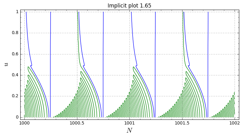
Is there possibly something wrong with the first term? Or is it related to the mod-part (that I have taken out).

[p15-git-acc]

I've added the right edge of the sharkfin, where the real part of -(c_0 a^{-1/3} + b^2 a^{-4/3} + 2\pi a^{-1/3}) ) is zero: To be clear, this is superimposed on the green plot of zeros of the real part of the Ht approximation, and also superimposed on the red plot of the left side of the shark fin where the magnitudes of the two summands of the approximation are equal.

[rudolph-git-acc]

This is a plot of the derivative of Im(S) (1.65 as per wiki, i.e. no terms removed except the mod):

[teorth]

Huh, it appears that there is some sort of "phase transition" near the right edge where just about anything we do to the imaginary part will pick up that edge.

The 2 Pi i N term in (1.65) can be replaced for instance by 2 Pi i {N} (at the cost of introducing one of these date line discontinuities). It's not so much the zero set of Im(S) that is relevant but more of a contour plot of when Im(S) hits a multiple of 2 Pi (or maybe Pi), as this should start creating the oscillations that one sees in the sharkfin.

p15's graph that Re( -(c_0 a^{-1/3} + b^2 a^{-4/3} + 2\pi a^{-1/3}) ) appears to change sign at the right edge of the sharkfin is convincing. I don't yet have a theoretical explanation as to why this ought to be the case, but assuming it we do at least have fairly short descriptions of both sides of the sharkfin now. One could now compute the point (N,u) where these two curves cross; this is something one could do for many ranges of N by computer rather than by eyeballing the sharkfin, and maybe we can start understanding the way in which u decays in N as well (this may help figure out how to do the asymptotics properly, since the first attempt I had was completely wrong).

[p15-git-acc]

One could now compute the point (N,u) where these two curves cross;

The point where the right edge curve intersects the vertical line past the top of the sharkfin could be interesting too, and probably even more tractable.

Edit: I think this vertical line intersection is u=pi*sqrt(32*(1-(1+sqrt(N^2-6*N+1))/N))

[teorth]

OK, I think I understand what is going on now.

The quantity (1.58) has two terms A+B, both involving an Airy function. But in the A term, the Airy function is applied to something with a positive real part and so there isn't much oscillation; in the B term, the Airy function is applied to something with a positive real part to the right of the right sharkfin edge and a negative real part to the left of this edge, so it oscillates to the left of this edge and doesn't oscillate to the right. This creates all the ridges in the zeros. But once one crosses the Re(S)=0 line, the amplitude of the oscillatory B term falls below that of the non-oscillatory A term and so now there are no more zeroes.

(I think a plot of Re(A) and Re(B) for a fixed choice of u, e.g., u=0.2, should illustrate the above behaviour.)

The right shark fin edge is basically a parabola in each strip corresponding to a fixed value of integer part [2N+1/2]; see (1.75) in the writeup.

Am still working on getting a good approximation to the left edge. EDIT: I now have a crude approximation, (1.82). The approximations suggest that actually (N, Nu^2) coordinates may give a better plot than (N,u) coordinates, in particular the (N,Nu^2) plot should be quite stable as one varies N (right now we are focusing on N ~ 1000, but I think the (N,Nu^2) plots for other values of N should give similar results).

[rudolph-git-acc]

That logic makes a lot of sense!

Here are the plots of the real parts of the A and B (approximate) Airy-functions as they appear in 1.58 with u fixed at 0.2:

[teorth]

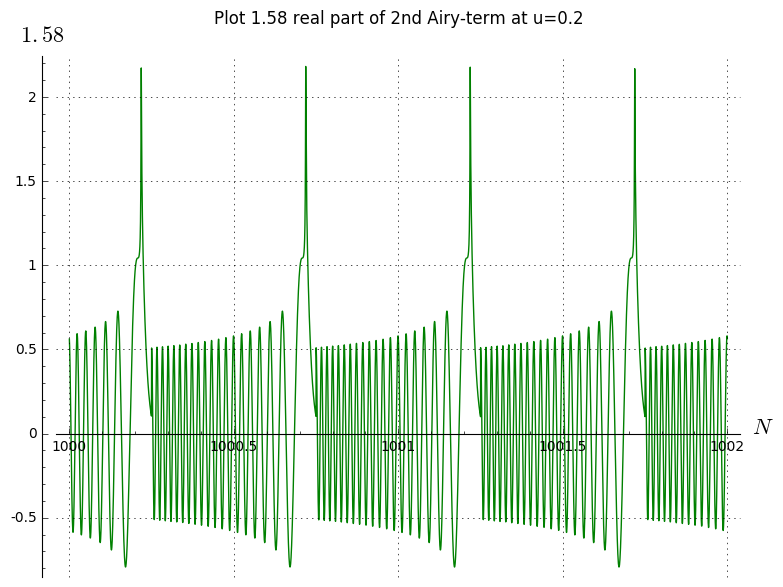
Thanks for the plots! (One could superimpose the first plot against the negative of the second plot to graphically illustrate where zeroes of the sum come from, but it's already clear what's going on from the two separate plots.) So inside the sharkfin, the first term is basically negligible and one is just seeing the zeroes of the Airy function of the second term.

As one increases u, the region where the oscillation of the second term dominates the magnitude of the first term shrinks, and at some point the sharkfin disappears and one either gets a lone zero (near the half-integers) or no zero (near the integers). I'm not sure exactly what the difference; the u=0.2 plots above seem to give no distinction between the half-integers and integers. But perhaps the situation will be clearer if we also make similar plots for higher values of u.

[p15-git-acc]

The approximations suggest that actually (N, Nu^2) coordinates may give a better plot than (N,u) coordinates

Here are plots of sign changes of the real part of (1.58) in the coordinates (N, v) where v=Nu^2.

N=[1000 - 1/4, 1000 + 1/4], v=[0, 300]:

N=[1000000 - 1/4, 1000000 + 1/4], v=[0, 300]:

In the second image the fin is mostly green with some patterns in the upper right and lower left. The upper right loops are real, but the patterns in the lower left are aliasing artifacts.

[rudolph-git-acc]

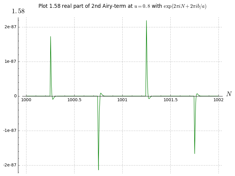
Here are a few more plots for the second Airy function at different u. Zeros indeed vanish when u increases.

[rudolph-git-acc]

The distinction between the half-integers and integers indeed doesn't come out from the graphs above, however when I include the weighting factor of exp(2*Pi*I*N +2*Pi*I*b(u)/a(N)) for the second Airy function, these patterns emerge:

[p15-git-acc]

The lighter part of this plot is supposed to be where the inequality (1.80) is true in N=[1000-1/4, 1000+1/4], v=[0, 300]:

It looks wrong, but I'm not sure if I wrote the code accurately.

[teorth]

Hmm, this looks weird... the LHS of (1.80) should be increasing as N increases (because c_0 becomes more and more negative), so the shaded region should be to the right of the curve rather than to the left. But the curve does seem to fit the sharkfin to first order on the left, it's the quadratic term that may need some correction. Perhaps if you post the code we could diagnose it? One could also try some earlier versions of this constraint (1.80) such as (1.77), (1.78), or (1.79).

[p15-git-acc]

The darker region is supposed to be where the inequality is false, but yeah I know it looks wrong. I mainly wanted to post it in case other people are making plots but not posting them because they are afraid they are wrong.

[p15-git-acc]

It looks like the b^2 ~ -(u^2)/16 approximation is too aggressive in the step from (1.77) to (1.78). Independent confirmation would be welcome!

(1.77):

(1.78):

[rudolph-git-acc]

If the main purpose of both conditions in 1.72 is to encapsulate the oscillations within a shark fin, then it appears that only evaluating 1.66 with the (simplified) condition 1.75 is already sufficient:

[rudolph-git-acc]

Here is the plot for 1.77:

and getting the same issue as P15 for 1.78:

which appears to be induced by a wrong sign before each Nu^2/(32pi) term in 1.78. Here is the plot with a minus sign before each of these factors:

EDIT: Working this through to 1.82 I get:

Ht182(N,u)=if(frac(2*N+1/2) > -N*u^2/(64*Pi^2)+(9/(256*Pi^2)*N*u^2)^(1/3),frac(2*N+1/2), 0)

which gives:

however with the corrected signs, the assumption in the step between 1.79 and 1.80 (on the region in 1.73) seems to be 'just true' for capturing the oscillations, but above those the red line now bends further backwards.

[teorth]

Thanks for fixing all the signs!

After all the approximations, the sharkfin region is now simplified to

(9 N u^2 / 256 Pi^2)^{1/3} - Nu^2/64 Pi^2 < { 2N + 1/2 } < 1 - Nu^2 /64 pi^2

so in particular the tip should be reached when

N u^2 = 256 Pi^2 / 9 ~ 280.7 {2N+1/2} = 5/9

which looks roughly in line with expectations (noting that our right edge of the sharkfin seems to extend by an extra wavelength or so from the last zero). Also if we use {2N+1/2}, Nu^2 coordinates (maybe using Nu^2/64 Pi^2 rather than Nu^2 is very slightly cleaner) then we now have determined the asymptotic shape of the sharkfin.

So I think we now have a pretty satisfactory description of the sharkfin region. As for the zeroes inside the sharkfin, we now know that the second term in (1.56) dominates, so I think more or less the zeroes should correspond to where (the real part of) -(c_0 a^{-1/3} + b^2 a^{-4/3} + 2 pi a^{-1/3}) matches a zero of the Airy function. These zeroes occur at -z where 2/3 z^{3/2} + pi/4 is close to a multiple of pi, so I guess the zeroes inside the sharkfin should be roughly where 2/3 (c_0 a^{-1/3} + b^2 a^{-4/3} + 2 pi a^{-1/3})^{3/2} + pi/4 is a multiple of pi? (I did some quick writeup on this on the wiki, may be sign errors though.)

[rudolph-git-acc]

This works great! Here are a few real zero trajectories computed by 1.89:

Since these curved trajectories are now numbered by n with n=1 being the most outer curve, does this mean we could calculate exactly how many of these curves will fit within a shark fin at a certain N?

[teorth]

Yes, I think so. As {2N+1/2} increases from 0 to 1, setting u=0 we see that the left-hand side of (1.89) decreases from (4/3) \sqrt{N} + 1/4 to 1/4. This suggests that there should be about (4/3) \sqrt{N} zeroes picked up, which from a visual count looks reasonably accurate (depending on what is going on at the bottom left corner of your more recent image).

On the other hand,the Riemann von Mangoldt formula tells us that the number of zeroes up to N at t=0 should be something like N^2 log N^2 - N^2, so in each interval [N - 1/4, N+1/4] there should actually be about 2 N log N zeroes initially. So only a small fraction of the zeroes are being part of this sharkfin - most of the zeroes are off doing something else, such as joining one of those complex curves we discovered previously.

It does occur to me though that one could at least hope to use this phenomena to give a proof that there are infinitely many zeroes of zeta on the critical line; there are other proofs of this type of result (and in fact a positive fraction of zeroes are known to be on the critical line) but I haven't seen an argument of this form before.

EDIT: the plots might look a bit straighter if one uses (N, Nu^2) (or N, Nu^2/64 pi^2) coordinates instead of (N,u) coordinates.

[rudolph-git-acc]

Using N, Nu^2/(64 pi^2)indeed straightens the plots quite a bit:

[rudolph-git-acc]

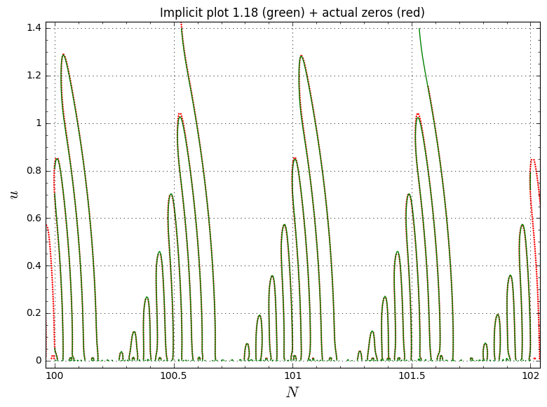
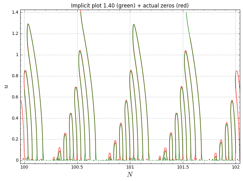
To check that we still have a reasonable fit with the actual zeros of Ht, over the last 4 days I have computed a larger set of zeros of eq 1.1 in the domain N=97...102, u = 0...1.4which roughly corresponds to x=125,000..139,000, t = -18,000...-100.

The results already look pretty good even at this relatively low size of N and we have seen improving asymptotics for higher N:

[p15-git-acc]

Here's what I get for (1.58) and (1.83) for N=[1000-1/4, 1000+1/4], w=N*u^2/(64*pi^2)=[0, 1/2]:

[rudolph-git-acc]

So only a small fraction of the zeroes are being part of this sharkfin - most of the zeroes are off doing something else, such as joining one of those complex curves we discovered previously.

In the spirit of 'all information about H_t originates from H_0', these straight vertical lines at the half integers actually do appear to send a tiny bit of information back to H_0, since two of these lines always seem to enclose an even number of zeros at t=0. I.e they can't just 'split up a pair of zeros' in their journey back to t=0 and have to pick their pass-through location with a certain care. Or, reasoning from t=0: does a zero att=0 already know it will stay single its entire life?