Resnet18-Cifar10分类

实验步骤

搭建resnet18网络

数据集加载

模型训练和改进

分析评估

Kaggle提交

网络构建

实验初期拟采用torchvision中实现的resnet18作为网络结构，为了方便修改网络结构，于是重新实现了resnet18网络

resnet18由一个7x7的降采样卷积，一个max pooling层，8个basicblock，一个全局池化层，最后接一个全连接层组成，如下图

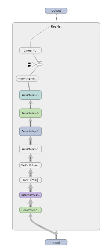
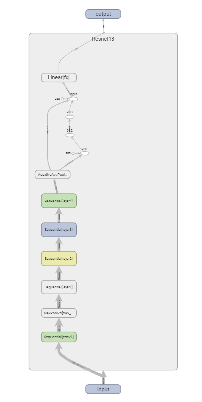
tensorboard网络结构可视化，左图为torchvision中的resnet实现，右图为自定义实现

代码如下

定义残差块

class IdentityBlock(nn.Module):
    def __init__(self, in_channels, out_channels, down_sampling=False):
        super().__init__()
        self.down_sampling = down_sampling
        self.in_channels = in_channels
        self.out_channels = out_channels
        self.conv1 = nn.Sequential(OrderedDict([
            ('conv1', nn.Conv2d(in_channels=in_channels, out_channels=out_channels, kernel_size=3,
                                stride=(1 if in_channels == out_channels else 2), padding=1,
                                bias=False)),
            ('bn1', nn.BatchNorm2d(out_channels)),
            ('relu1', nn.ReLU())
        ]))
        self.shortcut = nn.Sequential(OrderedDict([
            (
                'conv',
                nn.Conv2d(in_channels=in_channels, out_channels=out_channels, kernel_size=1, stride=2, bias=False)),
            ('bn', nn.BatchNorm2d(out_channels))
        ])) if in_channels != out_channels else nn.Sequential()
        self.conv2 = nn.Sequential(OrderedDict([
            ('conv2', nn.Conv2d(in_channels=out_channels, out_channels=out_channels, kernel_size=3, stride=1, padding=1,
                                bias=False)),
            ('bn2', nn.BatchNorm2d(out_channels))
        ]))
        self.relu2 = nn.ReLU()

    def forward(self, x):
        fx = self.conv1(x)
        fx = self.conv2(fx)
        x = self.shortcut(x)
        hx = fx + x
        hx = self.relu2(hx)
        return hx

定义模型网络

class Resnet18(nn.Module):
    def __init__(self, num_classes):
        super(Resnet18, self).__init__()
        self.conv1 = nn.Sequential(OrderedDict([
            ('conv', nn.Conv2d(in_channels=3, out_channels=64, kernel_size=7, stride=2, padding=3, bias=False)),
            ('bn', nn.BatchNorm2d(64)),
            ('relu', nn.ReLU()),
        ]))
        self.max_pool = nn.MaxPool2d(kernel_size=3, stride=2, padding=1)
        self.layer1 = self.make_layer(64, 64, down_sampling=False)
        self.layer2 = self.make_layer(64, 128)
        self.layer3 = self.make_layer(128, 256)
        self.layer4 = self.make_layer(256, 512)
        self.avg_pool = nn.AdaptiveAvgPool2d(output_size=(1, 1))
        self.fc = nn.Linear(in_features=512, out_features=num_classes)

    @staticmethod
    def make_layer(in_channels, out_channels, down_sampling=True):
        layer = nn.Sequential()
        layer.add_module('block1', IdentityBlock(in_channels, out_channels, down_sampling=down_sampling))
        layer.add_module('block2', IdentityBlock(out_channels, out_channels, down_sampling=False))
        return layer

    def forward(self, x):
        x = self.conv1(x)
        x = self.max_pool(x)
        x = self.layer1(x)
        x = self.layer2(x)
        x = self.layer3(x)
        x = self.layer4(x)
        x = self.avg_pool(x)
        x = x.view(x.size(0), -1)
        x = self.fc(x)
        return x

跟pytorch内置实现不同的是，在全局池化层后面pytorch采用了torch.flatten函数，而我是直接用了view方法。

数据集加载

数据集请前往kaggle官网下载 https://www.kaggle.com/c/cifar-10/data

下载完成后解压放置到dataset文件夹下，目录结构如下

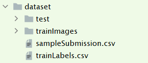
当然读者亦可使用torchvision内置的cifar10数据集，运行时会先下载cifar10数据集，可能下载比较慢，可以先运行一次，找到链接后自行下载完成后放到dataset文件夹下，然后重新运行

import torch
import torchvision
import torchvision.transforms as transforms

trainset = torchvision.datasets.CIFAR10(root='./dataset/cifar', train=True,
                                        download=True,transform=None)

testset = torchvision.datasets.CIFAR10(root='./dataset/cifar', train=False,
                                       download=True, transform=None)

数据集加载主要通过继承pytorch内置的dataset类，重写其中的__getitem__和__len__以及构造函数

我们读取训练集中的图片并划分成训练集和验证集。

__init__

class CifarDataset(Data.Dataset):
    def __init__(self, img_dir='dataset/trainImages/', train=True, img_label=None, transform=None):
        self.img_path = list(Path(img_dir).glob('*.png'))
        self.img_path.sort(key=lambda x: int(x.name.split('.')[0]))
        self.img_label = self.get_label(img_label)
        num_train = int(0.8 * len(self.img_path))
        index_list = list(range(len(self.img_path)))
        random.seed(42)
        indexes = random.sample(index_list, num_train)
        if not train:
            indexes = [index_list.pop(index) for index in indexes]
        self.img_path = [self.img_path[index] for index in indexes]
        self.img_label = [self.img_label[index] for index in indexes]
        self.transform = transform

上面的代码中get_label函数传入trainLabels.csv的路径，返回标签索引列表。img_path需要调用sort函数保证图片按id排序，这样才能和标签一一对应。在构造函数中，通过传入train参数决定加载训练集还是验证集，为了保证训练集和验证集不重复，设定随机种子以保证在构造训练集和验证集的两次随机操作中得到相同的索引。

    @staticmethod
    def get_label(label_path):
        if label_path is not None:
            df = pd.read_csv(label_path)
            class_dict = {label: i for i, label in enumerate(classes)}
            df['label'] = df['label'].apply(lambda x: class_dict[x])
            return list(df['label'].values)
        else:
            return None

传入transform，在__getitem__方法中对图片做预处理，img_label为None的情况是为了加载测试集（没有标签）

__getitem__

    def __getitem__(self, index):
        if self.img_label is not None:
            img = Image.open(self.img_path[index]).convert('RGB')
            label = np.array(self.img_label[index], dtype=int)
            if self.transform is not None:
                img = self.transform(img)
            return img, torch.from_numpy(label)
        else:
            img = Image.open(self.img_path[index]).convert('RGB')
            if self.transform is not None:
                img = self.transform(img)
            return img, torch.from_numpy(np.array([]))

__len__

    def __len__(self):
        return len(self.img_path)

调用

if __name__ == '__main__':
    transform_train = transforms.Compose([
        # 先填充，然后随机裁剪成32x32大小的图片
        transforms.RandomCrop(32, padding=4),
        # 图像一半的概率翻转，一半的概率不翻转
        transforms.RandomHorizontalFlip(),  
        transforms.ToTensor(),
        # R,G,B每层的归一化用到的均值和方差
        transforms.Normalize((0.4914, 0.4822, 0.4465), (0.2023, 0.1994, 0.2010)),
    ])

    transform_test = transforms.Compose([
        transforms.ToTensor(),
        transforms.Normalize((0.4914, 0.4822, 0.4465), (0.2023, 0.1994, 0.2010)),
    ])

    train_dataset = CifarDataset(img_dir='dataset/trainImages/', img_label='dataset/trainLabels.csv', train=True, transform=transform_train)
    val_dataset = CifarDataset(img_dir='dataset/trainImages/', img_label='dataset/trainLabels.csv', train=False, transform=transform_test)

模型训练

初始设置

设定随机种子，保证训练结果可浮现

def setup_seed(seed):
    torch.manual_seed(seed)
    torch.cuda.manual_seed_all(seed)
    np.random.seed(seed)
    random.seed(seed)
    torch.backends.cudnn.deterministic = True
# 设置随机数种子
setup_seed(hyp['random_seed'])

损失函数

交叉熵损失函数

# 定义损失函数
loss = nn.CrossEntropyLoss()

优化器

# 定义优化器
optimizer = optim.SGD(net.parameters(), lr=args.lr, momentum=args.momentum, weight_decay=args.weight_decay)

加载模型

if args.pretrained:
    model = resnet18(pretrained=False, num_classes=10)
    state_dict = torch.load('weights/resnet18-f37072fd.pth')
    state_dict.pop('fc.weight')
    state_dict.pop('fc.bias')
    model.load_state_dict(state_dict, strict=False)
elif args.my_resnet or args.my_improved:
    model = Resnet18(num_classes=10, improved=args.my_improved)
else:
    model = resnet18(pretrained=False, num_classes=10)

这里通过配置pretrained决定是否加载预训练权重。另外，pytorch内置resnet18最后一个全连接层是1000个输出，而分类cifar10我们需要设定全连接层为10个输出，所以我们加载权重的时候不加载全连接层的权重。

训练

best_acc = 0
# 开始训练
for epoch in range(hyp['init_epoch'], n_epoch):
    net.train()
    for X, y in tqdm(train_iter):
        X = X.to(device)
        y = y.to(device)
        y_hat = net(X)
        error = loss(y_hat, y).sum()
        error.backward()
        optimizer.step()
        optimizer.zero_grad()
    if hyp['scheduler']:
        scheduler.step()
    # 评估
    # ...
    # ...

评估

定义Metric类

每训练一轮，模型在验证集上进行评估，可利用sklearn.metrics实现准确率和f1-score的计算

import numpy as np
from sklearn.metrics import accuracy_score
from sklearn.metrics import f1_score

class Metric(object):
    def __init__(self, output, label):
        self.output = output
        self.label = label

    def accuracy(self):
        y_pred = self.output
        y_true = self.label
        y_pred = y_pred.argmax(dim=1)
        accuracy = accuracy_score(y_true, y_pred)
        return accuracy

    def f1_score(self, _type='micro'):
        y_pred = self.output
        y_true = self.label
        return f1_score(np.argmax(y_pred, 1), y_true, average=_type)

对于多元分类，f1-score的值跟accuracy是一样的，所以任意选择一个作为评估指标即可。

然而，我在看到图之后才意识到这一点，所以f1-score白算了

训练过程中的评估

    # 训练
    # ...
    net.eval()
    val_loss, val_acc, n = .0, .0, 0
    batch_count = 0
    for X, y in val_iter:
        X = X.to(device)
        y = y.to(device)
        y_hat = net(X)
        error = loss(y_hat, y).sum()
        val_loss += error.item()
        metric = Metric(y_hat.detach().cpu(), y.detach().cpu())
        val_acc += metric.accuracy()
        batch_count += 1
        n += y.shape[0]

    writer.add_scalar('val/loss', val_loss / n, epoch)
    writer.add_scalar('val/acc', val_acc / batch_count, epoch)
    print(f"epoch:{epoch} loss:{val_loss / n} acc:{val_acc / batch_count}")

保存模型

保存最佳准确率模型

    if (val_acc / batch_count) > max(best_acc, 0.7):
        best_acc = val_acc / batch_count
        with open(exp_dir + "/result.txt", mode='w') as f:
            f.write("best accuracy:" + str(best_acc) + "\n")
            f.write("epoch:" + str(epoch))
        torch.save(net.state_dict(), exp_dir + "/weights/best.pth")

保存最后一轮的模型

torch.save(net.state_dict(), exp_dir + "/weights/last.pth")

模型改进

网络改进

考虑到cifar10的图片尺寸太小，resnet18开头的7x7降采样卷积和池化容易丢失一部分信息，所以考虑将7x7的降采样和最大池化去掉，换成一个3x3的same卷积

if improved:
    self.conv1 = nn.Sequential(OrderedDict([
        ('conv', nn.Conv2d(in_channels=3, out_channels=64, kernel_size=3, stride=1, padding=1, bias=False)),
        ('bn', nn.BatchNorm2d(64)),
        ('relu', nn.ReLU())
    ]))
    self.max_pool = nn.MaxPool2d(kernel_size=3, stride=2, padding=1)
else:
    self.conv1 = nn.Sequential(OrderedDict([
        ('conv', nn.Conv2d(in_channels=3, out_channels=64, kernel_size=7, stride=2, padding=3, bias=False)),
        ('bn', nn.BatchNorm2d(64)),
        ('relu', nn.ReLU()),
    ]))

调整参数

本次调参主要调的是学习率，学习率的调整分两块，固定学习率调整和不固定的学习率调整。后者指的是学习率衰减

固定学习率

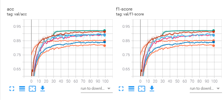
以下为学习率为0.1，0.01，0.001时训练100个epoch的曲线图

学习率衰减

采用multistep的学习率衰减策略

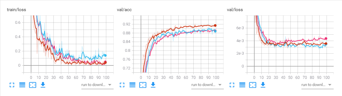
初始学习率为0.01，milestones = [30,60,90]，红色表示固定学习率

初始学习率为0.1，milestones = [30,60,90]，蓝色表示固定学习率

初始学习率为0.001，milestones = [30,60,90]，红色表示固定学习率

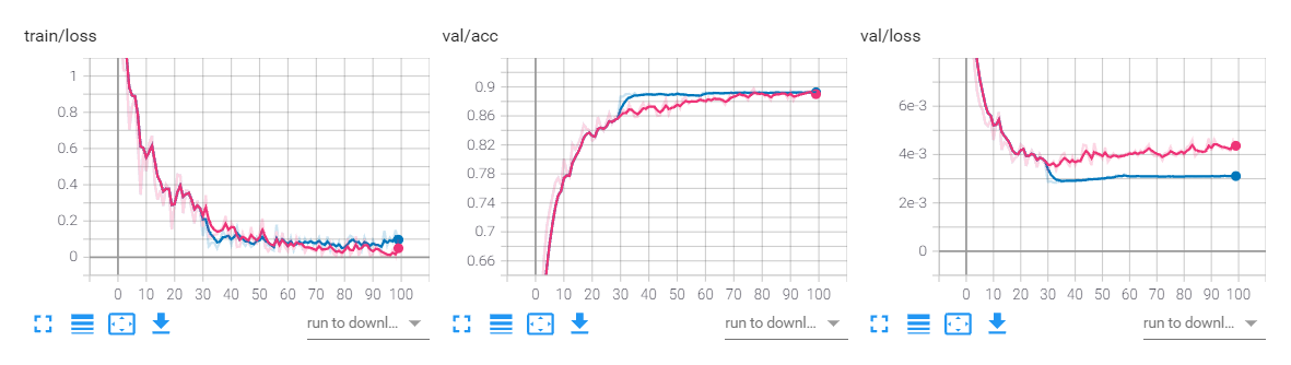
上述三种学习率情况下，都可以看出学习率衰减是有效的。

分析评估

run	exp	exp2	exp3	exp4	exp5	exp6	exp7	exp8	exp9
内置网络	√								√
自定义网络		√
自定义改进网络			√	√	√	√	√	√
预训练									√
学习率	0.01	0.01	0.01	0.1	0.001	0.01	0.1	0.001	0.01
学习率衰减						√	√	√
准确率	0.827	0.846	0.919	0.903	0.897	0.923	0.922	0.893	0.857

网络对比(exp,exp2,exp3)

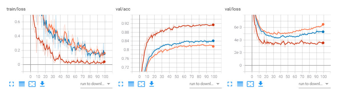
显然不管从图上还是表中都可以看出，自定义的resnet18略优于pytorch内置的resnet18，原因未知。而经过改进的网络更是显著由于前两者，首次将cifar10分类的准确率提升到了90以上。

学习率对比(exp3,exp4,exp5,exp6,exp7,exp8)

在前面模型改进-调参的地方已经提到没有应用学习率衰减的情况下，学习率为0.01比较合适。而且三个对比基本明学习率衰减有利于加速模型收敛，且设置合理的情况下可以增加准确率。

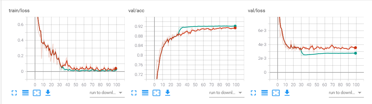
下图是学习率为0.01,0.1,0.001和三者是否使用学习率衰减的图

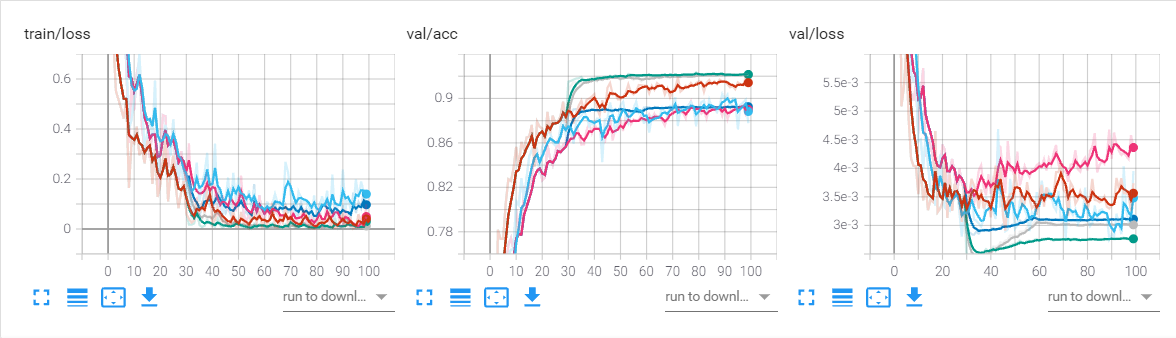
从图中可以看出。最优的是绿色曲线，即学习率为0.01且使用学习率衰减的情况。

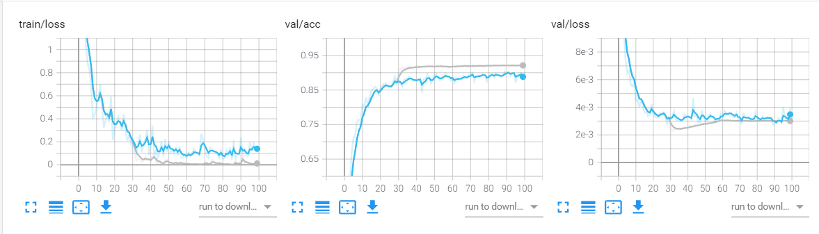
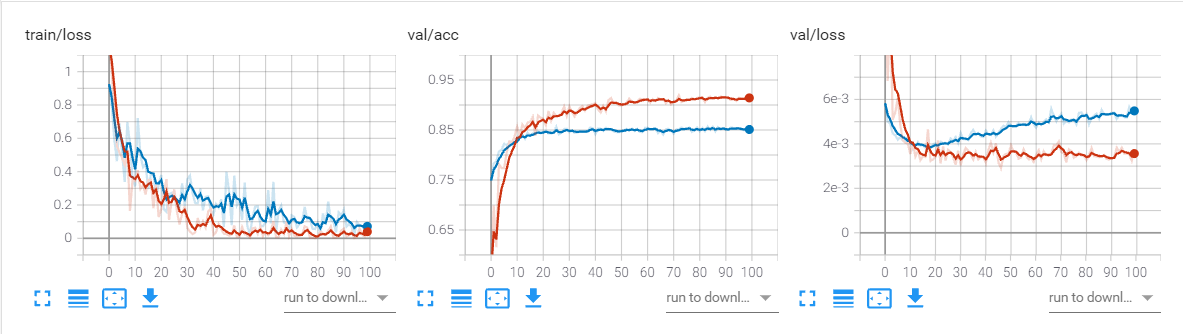
预训练对比(exp,exp9)

因为要使用预训练权重，我自己实现的resnet18的网络因为与内置网络存在差异，因此采用内置网络和加载预训练权重的内置网络作对比

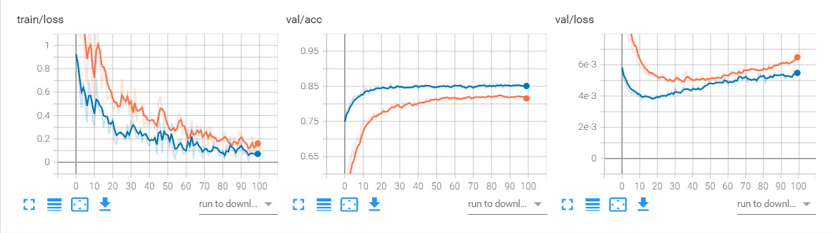
蓝色曲线表示加载预训练权重的网络。显然经过预训练的网络初始损失就较低且准确率较高，收敛速度和最终准确率都显著高于重头训练的网络。

预训练和网络结构的对比(exp3,exp9)

从上图可以看出，尽管经过预训练的网络初始准确率高，但是模型最终的表达能力仍然取决于网络结构。经过改进的网络即便没有经过预训练，最终的准确率较预训练的网络也提高了6.2个百分点，相较于没有经过预训练的内置网络提高了9.2个百分点

综上，当前最佳的模型为，自定义改进的网络在学习率为0.01时，经过[30,60,90]的multistep衰减，训练100轮的模型。

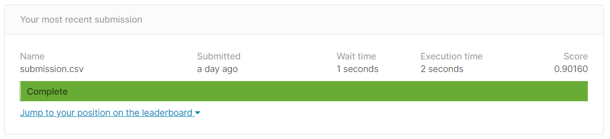
Kaggle提交