MFEM + PyMFEM (FEM library)
This repository provides Python binding for MFEM. MFEM is a high performance parallel finite element method (FEM) library (http://mfem.org/).
Installer (setup.py) builds both MFEM and binding together. By default, "pip install mfem" downloads and builds the serial version of MFEM and PyMFEM. Additionally, the installer supports building MFEM with specific options together with other external libraries, including MPI version.
Install
pip install mfem # binary install is available only on linux platforms (Py36-310)
Build with additional features (MPI, GPU, GPU-Hypre, GSLIB, SuiteSparse, libCEED, LAPACK)
The setup script accept various options. TO use it, one can either use --install-option flag
with pip, or download the package manually and run the script. For example, the one below downloads
and build parallel version of MFEM library (linked with Metis and Hypre)
and installs under
Build from local source file
# Download source and build
$ pip download mfem --no-binary mfem (expand tar.gz file and move to the downloaded directory)
or clone this repository
$ git clone https://github.com/mfem/PyMFEM.git

# Then, build it from local source
$ python -m pip install ./ --install-option="--with-parallel" --install-option="--mfem-branch=master"
or
$ python setup.py install --with-parallel # it download and build metis/hypre/mfem

# Verbose output
$ python setup.py install --verbose # SWIG output and CMAKE_VERBOSE_MAKEFILE is on

# Cleaning
$ python setup.py clean --all # clean external dependencies + wrapper code

# Choosing compiler
$ python setup.py install --with-parallel --CC=icc --CXX=icpc --MPICC=mpiicc --MPICXX=mpiicpc

# Run test
cd test
python test_examples.py -serial

# For other configurations, see docs/install.txt or help
$ python setup.py install --help
Usage
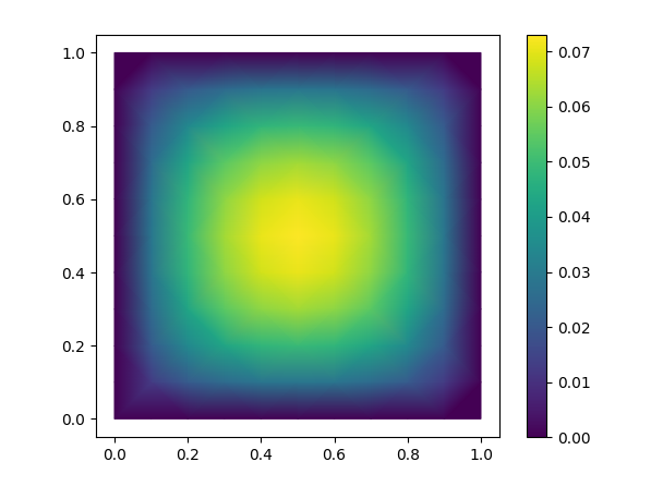
This example (modified from ex1.cpp) solves the Poisson equation,
$$\nabla \cdot (\alpha \nabla u) = f$$
in a square and plots the result using matplotlib.
Use the badge above to open this in Colab.
import mfem.ser as mfem

# Create a square mesh
mesh = mfem.Mesh(10, 10, "TRIANGLE")

# Define the finite element function space
fec = mfem.H1_FECollection(1, mesh.Dimension())   # H1 order=1
fespace = mfem.FiniteElementSpace(mesh, fec)

# Define the essential dofs
ess_tdof_list = mfem.intArray()
ess_bdr = mfem.intArray([1]*mesh.bdr_attributes.Size())
fespace.GetEssentialTrueDofs(ess_bdr, ess_tdof_list)

# Define constants for alpha (diffusion coefficient) and f (RHS)
alpha = mfem.ConstantCoefficient(1.0)
rhs = mfem.ConstantCoefficient(1.0)

"""
Note
-----
In order to represent a variable diffusion coefficient, you
must use a numba-JIT compiled function. For example:

>>> @mfem.jit.scalar
>>> def alpha(x):
>>>     return x+1.0
"""

# Define the bilinear and linear operators
a = mfem.BilinearForm(fespace)
a.AddDomainIntegrator(mfem.DiffusionIntegrator(alpha))
a.Assemble()
b = mfem.LinearForm(fespace)
b.AddDomainIntegrator(mfem.DomainLFIntegrator(rhs))
b.Assemble()

# Initialize a gridfunction to store the solution vector
x = mfem.GridFunction(fespace)
x.Assign(0.0)

# Form the linear system of equations (AX=B)
A = mfem.OperatorPtr()
B = mfem.Vector()
X = mfem.Vector()
a.FormLinearSystem(ess_tdof_list, x, b, A, X, B)
print("Size of linear system: " + str(A.Height()))

# Solve the linear system using PCG and store the solution in x
AA = mfem.OperatorHandle2SparseMatrix(A)
M = mfem.GSSmoother(AA)
mfem.PCG(AA, M, B, X, 1, 200, 1e-12, 0.0)
a.RecoverFEMSolution(X, b, x)

# Extract vertices and solution as numpy arrays
verts = mesh.GetVertexArray()
sol = x.GetDataArray()

# Plot the solution using matplotlib
import matplotlib.pyplot as plt
import matplotlib.tri as tri

triang = tri.Triangulation(verts[:,0], verts[:,1])

fig, ax = plt.subplots()
ax.set_aspect('equal')
tpc = ax.tripcolor(triang, sol, shading='gouraud')
fig.colorbar(tpc)
plt.show()
License
PyMFEM is licensed under BSD-3. Please refer the developers' web sites for the external libraries