thermox

This package provides a very simple interface to exactly simulate Ornstein-Uhlenbeck (OU) processes of the form

$$ dx = - A(x - b) dt + \mathcal{N}(0, D dt) $$

To collect samples from this process, define sampling times ts, initial state x0, drift matrix A, displacement vector b, diffusion matrix D and a JAX random key. Then run thermox.sample:

thermox.sample(key, ts, x0, A, b, D) 

Samples are then collected by exact diagonalization (therefore there is no discretization error) and JAX scans.

You can access log-probabilities of the OU process by running thermox.log_prob:

thermox.log_prob(ts, xs, A, b, D)

which can be useful for e.g. maximum likelihood estimation of the parameters A, b and D by composing with jax.grad.

Additionally thermox provides a scipy style suit of thermodynamic linear algebra primitives: thermox.linalg.solve, thermox.linalg.inv, thermox.linalg.expm and thermox.linalg.negexpm which all simulate an OU process under the hood. More details can be found in the thermo_linear_algebra.ipynb notebook.

Contributing

Before submitting any pull request, make sure to run pre-commit run --all-files.

Example usage

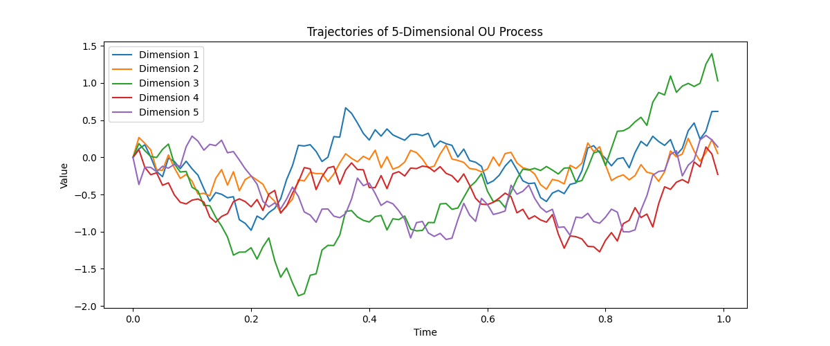
Here is a simple code example for a 5-dimensional OU process:

import thermox
import jax
import jax.numpy as jnp
import matplotlib.pyplot as plt

# Set random seed
key = jax.random.PRNGKey(0)

# Timeframe
dt = 0.01
ts = jnp.arange(0, 1, dt)

# System parameters for a 5-dimensional OU process
A = jnp.array([[2.0, 0.5, 0.0, 0.0, 0.0],
               [0.5, 2.0, 0.5, 0.0, 0.0],
               [0.0, 0.5, 2.0, 0.5, 0.0],
               [0.0, 0.0, 0.5, 2.0, 0.5],
               [0.0, 0.0, 0.0, 0.5, 2.0]])

b, x0 = jnp.zeros(5), jnp.zeros(5) # Zero drift displacement vector and initial state

 # Diffusion matrix with correlations between x_1 and x_2
D = jnp.array([[2, 1, 0, 0, 0],
               [1, 2, 0, 0, 0],
               [0, 0, 2, 0, 0],
               [0, 0, 0, 2, 0],
               [0, 0, 0, 0, 2]])

# Collect samples
samples = thermox.sample(key, ts, x0, A, b, D)

plt.figure(figsize=(12, 5))
plt.plot(ts, samples, label=[f'Dimension {i+1}' for i in range(5)])
plt.xlabel('Time')
plt.ylabel('Value')
plt.title('Trajectories of 5-Dimensional OU Process')
plt.legend()
plt.show()