Closed whedon closed 5 years ago
Hello human, I'm @whedon, a robot that can help you with some common editorial tasks. @dmbates, @ahwillia it looks like you're currently assigned to review this paper :tada:.
:star: Important :star:
If you haven't already, you should seriously consider unsubscribing from GitHub notifications for this (https://github.com/openjournals/joss-reviews) repository. As a reviewer, you're probably currently watching this repository which means for GitHub's default behaviour you will receive notifications (emails) for all reviews 😿
To fix this do the following two things:
For a list of things I can do to help you, just type:
@whedon commands
For example, to regenerate the paper pdf after making changes in the paper's md or bib files, type:
@whedon generate pdf
Attempting PDF compilation. Reticulating splines etc...
👋 @dmbates, @ahwillia — This is where the action happens. You both have a review checklist to work your way through. Feel free to post questions here and open review issues in the submission repository.
@dmbates, @ahwillia have you had a chance to look at this yet? 😄
I put it on my calendar for next Monday.
On Thu, Sep 5, 2019, 2:28 AM Olivia Guest notifications@github.com wrote:
@dmbates https://github.com/dmbates, @ahwillia https://github.com/ahwillia have you had a chance to look at this yet? 😄
— You are receiving this because you were mentioned. Reply to this email directly, view it on GitHub https://github.com/openjournals/joss-reviews/issues/1666?email_source=notifications&email_token=AAE3NUMAYYU4PDFC7GKFSLTQIDGM3A5CNFSM4IOF3FMKYY3PNVWWK3TUL52HS4DFVREXG43VMVBW63LNMVXHJKTDN5WW2ZLOORPWSZGOD56O5MQ#issuecomment-528281266, or mute the thread https://github.com/notifications/unsubscribe-auth/AAE3NUPTYBOUNTP7M22LAFLQIDGM3ANCNFSM4IOF3FMA .
I have finished the review of this paper and it looks very good to me. It is a pleasure to review a paper and software like this that has been so carefully created. My only comment is that the author has included the top-level Manifest.toml
file in the repository and I believe it is recommended not to do that. In other words, that name should be added to the .gitignore
file.
Thank you for the encouraging feedback, @dmbates.
I've added Manifest.toml
to the .gitignore
file. These changes are now implemented on the master branch and will be part of the next release.
Oh, one other thing I forgot to mention. I left the check box for version matches unchecked because the repository version is now ahead of the version given in the paper. I assume that the way to resolve this is to change the paper but I leave it to those who have more knowledge of the system to decide.
@labarba (please see comment directly above this) what do we do with different versions/how do we fix it? 😄
Once the review is finished, and all modifications done to the software and the paper, you ask the authors to make a new tagged release (and archive in Zenodo). You will then run the command:
@whedon set <v.x.x> as version
and the version number will be updated in the header comment here, and in the margin decorators of the first page of the paper in subsequent compilations.
I just want to echo all of @dmbates's positive comments. This is a very well done project and I think it should be accepted. Please treat the comments below as friendly suggestions and pointers for your future work.
I had one question when looking through the documentation. How do functions like cov(x, y)
and cor(x, y)
work if resample
is called independently on the x
and y
variables? It would seem like you'd need to specify a multivariate distribution (e.g. a bivariate Normal distribution) that specifies both x
and y
. Then you could call resample
once, and compute the correlation.
This package also takes a frequentist perspective. It could be nice to think about and maybe include a discussion in the documentation about how Bayesian statisticians would handle this problem. Their response would be to treat the data as fixed, and instead create a probabilistic model that captures the uncertainty. There are advantages/disadvantages associated with each approach. It's possible that the Bayesian approach is more computationally efficient on large-scale data—if I have a very large, uncertain dataset that takes a long time to fit, I'd need to resample my data many times and re-fit a very expensive model. In some cases the Bayesian model fitting can be faster, but is also typically very complicated and computationally intensive.
In case there is interest, here are some references on large-scale Bayesian model fitting:
I've checked all my boxes other than the release version number (as per above discussion).
🔔hey! @kahaaga have you had a chance to see the above? 😺
Thanks for the nice feedback and suggestions, @ahwillia!
cor(x,y) and related functions work
For the cov(x, y)
and cor(x, y)
functions, the approach is to always call resample
independently on x
and y
, because they might follow different distributions (hence, not necessarily normal distributions). The general approach (also for cor(x, y)
) is thus as follows.
Assume I have two uncertain datasets x
and y
of length n
, where element of the uncertain dataset is some distribution. Each element of x
, and each element of y
may be a regular numeric value with uncertainty, a normal distribution, an empirical distribution, a KDE to some distribution, a weighted population, or some new uncertain data type I choose to define, as long as I have a well-defined way of drawing random numbers from it.
To compute the correlation between x
and y
, I first resample x
according to the distributions furnishing it, and then resample y
according to the distributions furnishing it. That gives me one realization/draw for x
and one realization/draw for y
, both of length n
. The correlation between those two draws is then computed, yielding a single value for the correlation statistic. To get a distribution on the statistic, I just repeat that process many times.
This way, I can compute any statistic that accepts numerical vectors as inputs from uncertain data of any kind. For example, in the latest version of CausalityTools.jl, I use this approach to allow the user to compute various causality statistics from uncertain time series data.
I purposely went for this simplest possible approach. If your data is well-described by theoretical distributions, then you have the option to represent them as such. But if your data are not, then you still can handle uncertainties, because the resampling approach works where analytical expressions are hard to derive. In fact, the user already has the option to create a probabilistic model to represent their uncertainties, both using kernel density estimation and using model fitting. This is described in the documentation here.
If the user has some empirical distributions, they can use basic model fitting as such:
using Distributions, UncertainData
# Create a normal distribution
d = Uniform()
# Draw a 1000-point sample from the distribution.
some_sample = rand(d, 1000)
# Fitting a uniform distribution to the sample and treat the fitted model as
# our uncertain value.
uv = UncertainValue(Uniform, some_sample)
You can the access the fitted model by uv.distribution
, which on this particular random sample would give you a two-parameter model: FittedDistribution{Uniform{Float64}}(Uniform{Float64}(a=0.001019531622161507, b=0.998951965741667))
.
You could also fit a normal distribution by running
uv = UncertainValue(Normal, some_sample)
Again, accessing uv.distribution
gives you FittedDistribution{Normal{Float64}}(Normal{Float64}(μ=0.5005522321062404, σ=0.28621018213736704))
for this particular random vector.
These fitted models would be treated just as any other theoretical distribution, discrete population or other uncertain value types. The approach is always to resample. Hence, when doing
somesample1 = rand(10000)
somesample2 = rand(10000)
# Fit the data
uv1 = UncertainValue(Normal, some_sample)
uv2 = UncertainValue(Normal, some_sample)
# Resample uv1 and uv2 independetly, then compute the correlation on the draws
cor(uv1, uv2)
fitting is not done as part of the cor
computation. This is something the user would have
to do themselves before computing the correlation, if they desire to represent their data by a fitted model.
Although not implemented yet, Julia’s multiple dispatch may optionally be used to compute certain quantities in more efficient ways when there exists analytical expressions for the uncertain value type(s) involved. If some statistic f
is possible to compute analytically, it is of course possible to define f(type::T, x::FittedDistribution{Normal{Float64}}, y::FittedDistribution{Normal{Float64}}) where {T <: ExactComputationType}
. This way, you could provide an extra argument indicating that an exact computation method should be used. If some statistic requires fitting a bivariate normal distribution to x
, y
, then this would be the way to do it.
Just calling f(x, y)
, however, will always just resample x
and y
independently, then apply f
.
Does that answer your question, @ahwillia?
For now, only single model fits are possible. Distributions are as of now fitted using the machinery in Distributions.jl
, using maximum likehood estimation. More sophisticated model fitting schemes are possible to implement, which I guess is where some Bayesian statistics may come in handy (e.g. the Black Box Variational Inference algorithm (Ranganath et al. 2013) you mention). I am very excited about that idea.
I imagine having an UncertainValue
constructor with the signature UncertainValue(::SomeBayesianScheme, x::Vector{T}) where {T <: Real}
. Instead of returning a single fitted model, this constructor would perform model selection and represent the data using a class of models that have been selected based on whatever sampling scheme you provide.
Then, I guess that the user could do
# Pretend these are measured samples with an unknown distribution
somesample1 = rand(10000)
somesample2 = rand(10000)
# Set up some Bayesian analysis
model_scheme = SomeBayesianScheme()
# Fit models to each of the measured samples using the Bayesian scheme
uval1 = UncertainValue(model_scheme, somesample1)
uval2 = UncertainValue(model_scheme, somesample2)
This constructor could return an instance of a new type, e.g. SomeBayesianEstimate
, that contains the constructed model. The user could then do
uval1.model
uval2.model
to access the constructed models. Resampling those models is just then a matter of defining resample(uval::SomeBayesianEstimate)
, which would sample from the class of fitted models according to some criteria.
This would be an incredibly powerful tool, because you could start mixing different model fitting methods. For example:
# Pretend these are measured samples with an unknown distribution
somesample1 = rand(10000)
somesample2 = rand(10000)
uval1 = UncertainValue(Normal, somesample1)
uval2 = UncertainValue(FancyBayesianScheme(), somesample2)
# Compute some statistic `f` between the two samples assuming that the first one
# is well-approximated by a Normal distribution, while the second is represented
# by a class of models derived using a Bayesian method. This would work seamlessly,
# because `resample` would be called independently on `uval1` and `uval2`.
f(uval1, uval2)
Thus, the resampling machinery already implemented lends itself naturally to the Bayesian approach. Although this approach is not implemented yet, it is definitiely an interesting potential future development.
I’ve had a brief look at the papers you suggested, @ahwillia, but they are pretty dense. Bayesian statistics is relatively new to me, and I imagine it would take a considerable effort to get my understanding of these methods to a level where I can implement them or write something reasonable about them.
Considering that fitted models is just one of many ways to represent uncertain data in the package, I am a bit hesitant to spend a lot of time on this for the current version of the package. Was your intention that a frequentist vs. Bayesian discussion needs to be included in the current release before publication of the paper, or just a hint about possible future evolution of the package documentation, @ahwillia?
Maybe improving the section on model fitting (in the documentation, this now lies under "Uncertain Values" -> "Representations" -> "Theoretical distributions with fitted parameters") is sufficient, mentioning that other approaches is possible to implement? Any thoughts?
In summary, by using the resampling approach, combining quantitative constraints (i.e. theoretical distributions) and qualitative constraints (expert opinion) can be done seamlessly. This gives the user a tool to incorporate everything they know about their data, quantitatively and qualitatively, in their analysis. In the preprocessing stage, this can involve any kind of model fitting (if implemented) or expert judgement. You might even think about a scenario where you apply two separate Bayesian model fitting algorithms, yielding two separate classes of models, then treating these as a two-element population. During resampling, you can then draw values from the space of both models, but weight the probability of drawing from the models of a particular algorithm according to how much you trust the algorithm.
This approach is common in the field of paleoclimate science, where different proxy records (with different types of uncertainties and different magnitudes of uncertainties) representing the same physical process are often mixed to create a single proxy record for some phenomenon. For example, proxy data values may be well-explained by some class of models, but weighting the models to create the final, single record requires expert opinion on the proxy methods and analytical approaches.
One question, @oliviaguest:
@kahaaga nice — thanks! So does what @labarba said above not apply here regarding a new version: https://github.com/openjournals/joss-reviews/issues/1666#issuecomment-529135663?
@oliviaguest, you are absolutely right, it does apply here! My bad :)
I guess it would be nice that the release that is tagged in the paper also contains the latest version of the paper. The process for registering a new version of a package consists of the following steps:
This process may take a few days, depending on how busy the maintainers of the main repo are.
So I guess the process is: make any changes/additions @ahwillia wants, or other additions/changes, to the paper and/or documentation. Then, if the paper is accepted, release new version. Finally, trigger whedon-bot after the tagbot has made a new release, so that this is what goes into the final pdf?
Great! 😊 So regrading what needs to be done: I believe so, yes. Post back here when you think it's all ready.👍
Perfect, and thanks for the swift replies! This review process is new to me, so I just needed to be sure that I understand the process properly.
I'll post back once @ahwillia has responded to my comments and I've incorporated any final changes.
Thanks for the detailed response! No need to change anything with regard to Bayesian methods. I just wanted to mention it as a different perspective (it is not clear to me one is better than the other). Also -- I apologize, my recommended papers were not chosen very well. I would start with Murphy's textbook particularly the section on Bayesian model selection.
Re: corr and cov functions. You are assuming that x
and y
are independent then, p(x, y) = p(x) * p(y)
. If x
and y
are both univariate normals the correlation/covariance will always be zero, but for other distributions this may not be the case. Am I understanding correctly? If so, perhaps the assumption of independence should be stated?
Thanks for the reference to Murphy's textbook. Although model fitting is not the main focus of this package, bayesian model selection would be an interesting feature to have when the user wants to model their empirical distributions (beyond what is already possible in the package). I'll check the book and the papers you cited in more detail .
cor
and cov
Actually, neither cor
nor cov
are implemented for single uncertain values, only for uncertain datasets . The function signature for the correlation is nowcor(d1::AbstractUncertainValueDataset, d2::AbstractUncertainValueDataset, n::Int)
.
That is, they are computed on draws from collections of different values, where each value in the collection can be certain (e.g. a scalar) or uncertain (theoretical normal distribution, a fitted distribution, a population, etc).
This would be the equivalent of having, say, two time series with uncertainties in the measured values. Maybe the magnitudes of the uncertainties fluctuate through time, so at each instant of time there is a different distribution representing the value.
If I wanted point estimates on a statistic f
, I could just define a method f(uval1::AbstractUncertainValue, uval2::AbstractUncertainValue, n::Int)
that computes the correlation between two single uncertain values uval1
and uval2
by resampling them independently n
time, then computing f
on the draws. I describe how to do this in the documentation.
For example, define cor(uval1::AbstractUncertainValue, uval2::AbstractUncertainValue, n::Int)
as
import Statistics: cor
function cor(uval1::AbstractUncertainValue, uval2::AbstractUncertainValue, n::Int)
cor(resample(uval1, n), resample(uval2, n))
end
Which we can use like this:
# Point-estimate of correlation between a gamma distribution and a
# three-member weighted population with relative probabilities 0.3, 0.3 and 0.4
cor(UncertainValue(Gamma, 1, 2), UncertainValue([1.1, 2.2, 3.3], [0.3, 0.3, 0.4]), 100)
> 0.007348007353157689
# Point-estimate of the correlation between two normal distributions
cor(UncertainValue(Normal, 0, 1), UncertainValue(Normal, 4.2, 0.5), 10000)
> -0.002492518462927909
# Define a mixture model of a bunch of different distributions, and sample this
# to simulate some measured value with complicated uncertainty
M1 = MixtureModel([Beta(0.5, 1), Normal(-3, 0.5), Normal(2, 1), Normal(5, 2), Gamma(1, 2)])
empirical_sample = rand(M1, rand(5000:10000))
# Point-estimate of the correlation between this empirical sample and a
# beta distribution (calling UncertainValue(empirical_sample) triggers a KDE estimate
# to the distribution.
cor(UncertainValue(empirical_sample), UncertainValue(Beta, 2, 5), 10000)
> 0.013776522799511042
Hence, I get a point estimate for my statistic that is the result of sampling each value n=10000
times, then computing the correlation between those two 10000
-member distributions.
Here, I assume nothing other than that uval1
and uval2
must be sampled independently to not induce any correlation that is not present.
This is different from computing the correlation between two uncertain datasets, which I describe below.
using UncertainData, Distributions
# Simulate some mean data values measured for two phenomena (whatever they are)
values_var1 = sin.(0:0.1:10)
values_var2 = cos.(0:0.1:10)
If we wanted, we could now directly compute the correlation between the two time series
by calling cor(values_var1, values_var2)
. This would yield a single estimate of the correlation statistic:
cor(values_var1, values_var2)
> 0.0548362735517299
But instead, let's imagine that we also had access to information about uncertainties on the measure data values.
# Assume the data were measured by a device with normally distributed measurement uncertainties with fluctuating standard deviations in the following range
σ_range = (0.1, 0.7)
Now, how do we compute the correlation between the two series, when each of them have uncertainties associated with each point in the time series? The answer (in this package) is to resample.
# Instead of working with just the means, let's instead work with each point as
# a normal distribution.
uncertain_vals1 = [UncertainValue(Normal, val, rand(Uniform(σ_range...))) for val in values_var1]
uncertain_vals2 = [UncertainValue(Normal, val, rand(Uniform(σ_range...))) for val in values_var2]
# Convert to `UncertainValueDataset`s, so that we can call `cor`
uncertain_dataset1 = UncertainValueDataset(uncertain_vals1)
uncertain_dataset2 = UncertainValueDataset(uncertain_vals2)
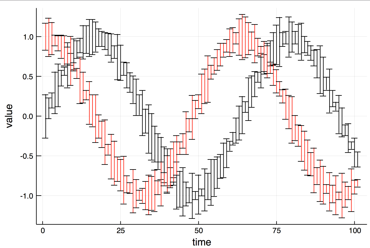
Plotting the data:
Now, draw one realisation of uncertain_dataset1
in an element-wise manner (one draw from each distribution furnishing the dataset). Next, draw an independent realisation of uncertain_dataset2
the same way. Finally, compute the correlation between these two realisations. The function signature for the correlation is nowcor(d1::AbstractUncertainValueDataset, d2::AbstractUncertainValueDataset, n::Int)
, so to estimate the correlation for a single draw, you´d do
cor(uncertain_dataset1, uncertain_dataset2, 1)
which would give you a single estimate for the correlation. Repeating that many times, we get a distribution of estimates for the correlation:
cor(uncertain_dataset1, uncertain_dataset2, 10000)
Plotting the histogram of the distribution of correlation estimates, we get a mean correlation estimate close to the estimate for the time series without uncertainties.
Thus, there's nothing special about cor
or cov
. Using this resampling strategy, any other quantity or statistic can be computed in a similar manner. This is exactly the same approach I use in CausalityTools
to obtain confidence intervals on the various statistical estimators of dynamical coupling, which are alternative ways of analyzing time series like this.
Of course, the interpretation of the results is something else entirely, and here you'd have think about underlying assumptions. One can always use this resampling approach to compute anything. How meaningful it is to do so for a given statistic, such as the correlation, is a different question. It is the user's responsibility to know the limitations of the statistical estimators they apply, what they mean, and how applicable the method is to their data.
The advantage of this approach is that it separates the analysis into distinct stages for the user:
Define the empirical distributions, weighted populations, fitted distributions or theoretical distributions representing the possible values in the dataset. Here, you can incorporate most of the prior information you have about your data.
Implement the statistic you're interested in for vector-valued inputs.
Make a wrapper around the function for the statistic that accepts uncertain datasets as inputs.
Repeat the computation for multiple realisations of your dataset. Resampling many times, we get a distribution over the statistic, from which we can obtain confidence intervals on the statistic.
In the resampling stage, you can also input other prior information, such as "I only want to sample the indices of my dataset such that they are strictly increasing". The statistic is then computed over the draws, and we get a estimated distribution over the value of the statistic. This distribution then encompasses all the prior information you had on uncertainties and on sampling constraints that you applied during the resampling process.
Does this answer your question?
I will implement the cor(x::AbstractUncertainValue, y::AbstractUncertainValue, n::Int)
method as described above as part of the next release (so that it gets into the version that goes with the paper).
Although the information is already present in the documentation, I think it is a good idea to make some tutorials that describes this more thoroughly, like in this answer. I'll create an issue in the github repository that tracks this.
Interesting -- thanks for putting so much effort into this. I like the goal of breaking it down into 4 steps for the user.
Here, I assume nothing other than that uval1 and uval2 must be sampled independently
^ This was all I was after. I think if you don't make some sort of assumption like this, it can be a hard problem.
For example, you could think of drawing n
observations from a multivariate Gaussian distribution. Say this results in a data matrix with shape n x m
.
Then, one could fit the mean and covariance matrix to those data to estimate the underlying distribution.
Now, when you call resample
, I suppose it would return entire rows (length-m
) vectors. By doing this it would capture correlations amongst the m
variables, which wouldn't be possible if you resampled each of the m
columns independently. In this case the columns are not independent of each other due to the correlations induced by the covariance matrix.
Of course, the interpretation of the results is something else entirely, and here you'd have think about underlying assumptions. One can always use this resampling approach to compute anything. How meaningful it is to do so for a given statistic, such as the correlation, is a different question. It is the user's responsibility to know the limitations of the statistical estimators they apply, what they mean, and how applicable the method is to their data.
I agree with this, assuming that resample
draws an actual sample from the true underlying distribution of the data. So all I request is that the assumptions are stated in the tutorials.
For example, the fact that noise is applied elementwise in the time series example is an assumption. Alternatively, one could fit a Gaussian process model to the data. Resamples from this model would be very different than resamples from the i.i.d. noise model you suggest.
Thanks again for putting time into making detailed tutorials for your package. Again, I am signed off for this to be accepted.
@kahaaga hi there, what is left to be done to the code and in general from your end? 😊
I've now re-done the entire documentation for the package to make the points that @ahwillia pointed out much more clear. Instead of making tutorials explaining the difference (which might be missed by users unless they really dive into the documentation), I now explain the resampling procedure in detail for each function that uses it.
Concretely, this involved re-working the documentation for the statistical functions from scratch, adding detailed sections on how each of the computations are done. Moreover, I added a section on the difference between exact error propagation and approximate error propagation used in this package. I'll add tutorials later, but that is a bit beyond the scope of the software itself. It should be clear for the user what assumptions goes into the computations now.
I hope that satisfactorily addresses your comments, @ahwillia.
As for the code, I've submitted version 0.5.0 (which incorporates the above changes and some more) to the Julia registry. If everything goes fine, the new version should be registered and tagged within a day or two. Once the process is finished, I'll tag you here, @oliviaguest.
Looks good to me!
On Wed, Oct 9, 2019, 1:33 AM Kristian Agasøster Haaga < notifications@github.com> wrote:
I've now re-done the entire documentation for the package to make the points that @ahwillia https://github.com/ahwillia pointed out much more clear. Instead of making tutorials explaining the difference (which might be missed by users unless they really dive into the documentation), I now explain the resampling procedure in detail for each function that uses it.
Concretely, this involved re-working the documentation for the statistical functions from scratch, adding detailed sections on how each of the computations are done. Moreover, I added a section on the difference between exact error propagation and approximate error propagation used in this package. I'll add tutorials later, but that is a bit beyond the scope of the software itself. It should be clear for the user what assumptions goes into the computations now.
I hope that satisfactorily addresses your comments, @ahwillia https://github.com/ahwillia.
As for the code, I've submitted version 0.5.0 (which incorporates the above changes and some more) to the Julia registry. If everything goes fine, the new version should be registered and tagged within a day or two. Once the process is finished, I'll tag you here, @oliviaguest https://github.com/oliviaguest.
— You are receiving this because you were mentioned. Reply to this email directly, view it on GitHub https://github.com/openjournals/joss-reviews/issues/1666?email_source=notifications&email_token=AAE3NUKMARTHDWU2G7AJNTLQNWJOFA5CNFSM4IOF3FMKYY3PNVWWK3TUL52HS4DFVREXG43VMVBW63LNMVXHJKTDN5WW2ZLOORPWSZGOEAXDDFI#issuecomment-539898261, or mute the thread https://github.com/notifications/unsubscribe-auth/AAE3NUK5YV6BASKYG4MADBTQNWJOFANCNFSM4IOF3FMA .
@oliviaguest The newest version of my package has been registered in the Julia repository and tagged with version 0.5.1 (see release list). I don't have more to add at this stage, so all should be ready for re-generating the pdf!
@whedon generate pdf
Attempting PDF compilation. Reticulating splines etc...
@kahaaga looks good to me, what do you think?
@dmbates @ahwillia I think you can now tick the last box? :smile:
Looks good to me!
@oliviaguest Is there anything left for me to do here?
@kahaaga no, thank you.
@labarba do we need the reviewers to tick this final box? 🤔
@oliviaguest Having all the boxes checked is preferable, but it is clear this has been taken care of so the review can move forward. Do you want to go ahead and update the version number? Looks like it has continued to be updated in the meantime.
@kahaaga Which version of your package do you intend to be associated with the JOSS paper?
The latest release of the package is v0.8.2 and the functionality is still the same (but with some additional minor features), so I guess the latest version could be associated with the paper?
I finally remembered to check the box on the version for my review. It's all good to go as far as I am concerned.
@oliviaguest When a reviewer misses to tick the version box, and I (as handling editor) have checked the version, the I actually click the box myself to complete the checklist.
Thanks all! So @labarba by check do you mean check if the version in this issue (text at the top) matches that in the code? And do I change it just by editing the text above?
Authors need to make a tagged release of their software to include the latest revisions. The version number will thus increase. You, as handling editor, run @whedon set v.xx as version
. That will update the version at the top of this issue, and then you are done, and can check off the item on the checklist.
@whedon set v0.8.2 as version
OK. v0.8.2 is the version.
@whedon generate pdf
Attempting PDF compilation. Reticulating splines etc...
hey @kahaaga — can you please create an archive for the code (on Zenodo, figshare, etc.) and post the archive DOI here so we can get this published? :smile:
@oliviaguest I've archived the software at Zenodo and added the DOI (10.5281/zenodo.3522252) to the README . Should be good to go now!
@whedon set 10.5281/zenodo.3522252 as archive
OK. 10.5281/zenodo.3522252 is the archive.
@whedon accept
Attempting dry run of processing paper acceptance...
Submitting author: @kahaaga (Kristian Agasøster Haaga) Repository: https://github.com/kahaaga/UncertainData.jl Version: v0.8.2 Editor: @oliviaguest Reviewer: @dmbates, @ahwillia Archive: 10.5281/zenodo.3522252
Status
Status badge code:
Reviewers and authors:
Please avoid lengthy details of difficulties in the review thread. Instead, please create a new issue in the target repository and link to those issues (especially acceptance-blockers) by leaving comments in the review thread below. (For completists: if the target issue tracker is also on GitHub, linking the review thread in the issue or vice versa will create corresponding breadcrumb trails in the link target.)
Reviewer instructions & questions
@dmbates & @ahwillia, please carry out your review in this issue by updating the checklist below. If you cannot edit the checklist please:
The reviewer guidelines are available here: https://joss.readthedocs.io/en/latest/reviewer_guidelines.html. Any questions/concerns please let @oliviaguest know.
✨ Please try and complete your review in the next two weeks ✨
Review checklist for @dmbates
Conflict of interest
Code of Conduct
General checks
Functionality
Documentation
Software paper
paper.md
file include a list of authors with their affiliations?Review checklist for @ahwillia
Conflict of interest
Code of Conduct
General checks
Functionality
Documentation
Software paper
paper.md
file include a list of authors with their affiliations?