robertmartin8/PyPortfolioOpt

PyPortfolioOpt is a library that implements portfolio optimization methods, including classical mean-variance optimization techniques and Black-Litterman allocation, as well as more recent developments in the field like shrinkage and Hierarchical Risk Parity.

It is extensive yet easily extensible, and can be useful for either a casual investors, or a professional looking for an easy prototyping tool. Whether you are a fundamentals-oriented investor who has identified a handful of undervalued picks, or an algorithmic trader who has a basket of strategies, PyPortfolioOpt can help you combine your alpha sources in a risk-efficient way.

PyPortfolioOpt has been published in the Journal of Open Source Software 🎉

PyPortfolioOpt is now being maintained by Tuan Tran.

Head over to the documentation on ReadTheDocs to get an in-depth look at the project, or check out the cookbook to see some examples showing the full process from downloading data to building a portfolio.

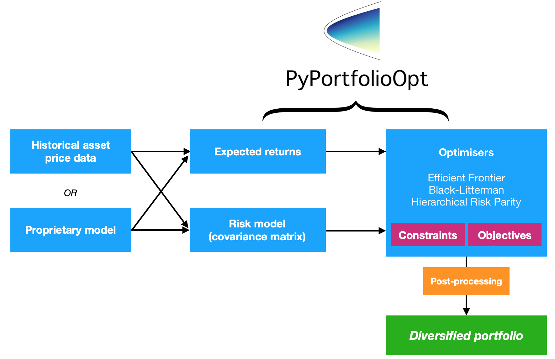
Table of contents
Getting started
- For development
A quick example
An overview of classical portfolio optimization methods
Features
Advantages over existing implementations
Project principles and design decisions
Testing
Citing PyPortfolioOpt
Contributing
Getting in touch

Getting started

If you would like to play with PyPortfolioOpt interactively in your browser, you may launch Binder here. It takes a while to set up, but it lets you try out the cookbook recipes without having to deal with all of the requirements.

Note: macOS users will need to install Command Line Tools.

Note: if you are on windows, you first need to installl C++. (download, install instructions)

This project is available on PyPI, meaning that you can just:

pip install PyPortfolioOpt

(you may need to follow separate installation instructions for cvxopt and cvxpy).

However, it is best practice to use a dependency manager within a virtual environment. My current recommendation is to get yourself set up with poetry then just run

poetry add PyPortfolioOpt

Otherwise, clone/download the project and in the project directory run:

python setup.py install

PyPortfolioOpt supports Docker. Build your first container with docker build -f docker/Dockerfile . -t pypfopt. You can use the image to run tests or even launch a Jupyter server.

# iPython interpreter:
docker run -it pypfopt poetry run ipython

# Jupyter notebook server:
docker run -it -p 8888:8888 pypfopt poetry run jupyter notebook --allow-root --no-browser --ip 0.0.0.0
# click on http://127.0.0.1:8888/?token=xxx

# Pytest
docker run -t pypfopt poetry run pytest

# Bash
docker run -it pypfopt bash

For more information, please read this guide.

For development

If you would like to make major changes to integrate this with your proprietary system, it probably makes sense to clone this repository and to just use the source code.

git clone https://github.com/robertmartin8/PyPortfolioOpt

Alternatively, you could try:

pip install -e git+https://github.com/robertmartin8/PyPortfolioOpt.git

A quick example

Here is an example on real life stock data, demonstrating how easy it is to find the long-only portfolio that maximises the Sharpe ratio (a measure of risk-adjusted returns).

import pandas as pd
from pypfopt import EfficientFrontier
from pypfopt import risk_models
from pypfopt import expected_returns

# Read in price data
df = pd.read_csv("tests/resources/stock_prices.csv", parse_dates=True, index_col="date")

# Calculate expected returns and sample covariance
mu = expected_returns.mean_historical_return(df)
S = risk_models.sample_cov(df)

# Optimize for maximal Sharpe ratio
ef = EfficientFrontier(mu, S)
raw_weights = ef.max_sharpe()
cleaned_weights = ef.clean_weights()
ef.save_weights_to_file("weights.csv")  # saves to file
print(cleaned_weights)
ef.portfolio_performance(verbose=True)

This outputs the following weights:

{'GOOG': 0.03835,
 'AAPL': 0.0689,
 'FB': 0.20603,
 'BABA': 0.07315,
 'AMZN': 0.04033,
 'GE': 0.0,
 'AMD': 0.0,
 'WMT': 0.0,
 'BAC': 0.0,
 'GM': 0.0,
 'T': 0.0,
 'UAA': 0.0,
 'SHLD': 0.0,
 'XOM': 0.0,
 'RRC': 0.0,
 'BBY': 0.01324,
 'MA': 0.35349,
 'PFE': 0.1957,
 'JPM': 0.0,
 'SBUX': 0.01082}

Expected annual return: 30.5%
Annual volatility: 22.2%
Sharpe Ratio: 1.28

This is interesting but not useful in itself. However, PyPortfolioOpt provides a method which allows you to convert the above continuous weights to an actual allocation that you could buy. Just enter the most recent prices, and the desired portfolio size ($10,000 in this example):

from pypfopt.discrete_allocation import DiscreteAllocation, get_latest_prices

latest_prices = get_latest_prices(df)

da = DiscreteAllocation(weights, latest_prices, total_portfolio_value=10000)
allocation, leftover = da.greedy_portfolio()
print("Discrete allocation:", allocation)
print("Funds remaining: ${:.2f}".format(leftover))

12 out of 20 tickers were removed
Discrete allocation: {'GOOG': 1, 'AAPL': 4, 'FB': 12, 'BABA': 4, 'BBY': 2,
                      'MA': 20, 'PFE': 54, 'SBUX': 1}
Funds remaining: $11.89

Disclaimer: nothing about this project constitues investment advice, and the author bears no responsibiltiy for your subsequent investment decisions. Please refer to the license for more information.

An overview of classical portfolio optimization methods

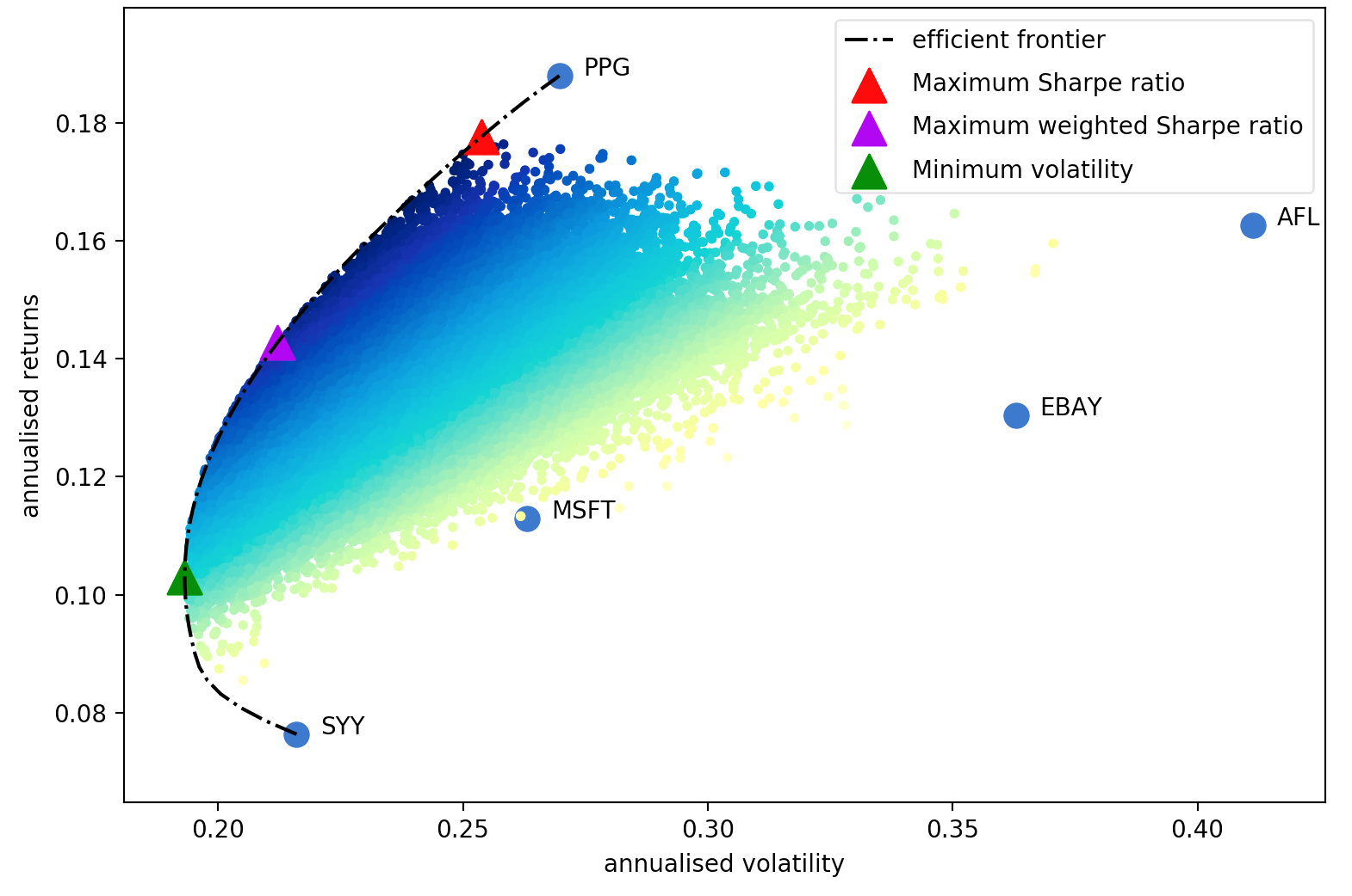
Harry Markowitz's 1952 paper is the undeniable classic, which turned portfolio optimization from an art into a science. The key insight is that by combining assets with different expected returns and volatilities, one can decide on a mathematically optimal allocation which minimises the risk for a target return – the set of all such optimal portfolios is referred to as the efficient frontier.

Although much development has been made in the subject, more than half a century later, Markowitz's core ideas are still fundamentally important and see daily use in many portfolio management firms. The main drawback of mean-variance optimization is that the theoretical treatment requires knowledge of the expected returns and the future risk-characteristics (covariance) of the assets. Obviously, if we knew the expected returns of a stock life would be much easier, but the whole game is that stock returns are notoriously hard to forecast. As a substitute, we can derive estimates of the expected return and covariance based on historical data – though we do lose the theoretical guarantees provided by Markowitz, the closer our estimates are to the real values, the better our portfolio will be.

Thus this project provides four major sets of functionality (though of course they are intimately related)

Estimates of expected returns
Estimates of risk (i.e covariance of asset returns)
Objective functions to be optimized
Optimizers.

A key design goal of PyPortfolioOpt is modularity – the user should be able to swap in their components while still making use of the framework that PyPortfolioOpt provides.

Features

In this section, we detail some of PyPortfolioOpt's available functionality. More examples are offered in the Jupyter notebooks here. Another good resource is the tests.

A far more comprehensive version of this can be found on ReadTheDocs, as well as possible extensions for more advanced users.

Expected returns

Mean historical returns:
- the simplest and most common approach, which states that the expected return of each asset is equal to the mean of its historical returns.
- easily interpretable and very intuitive
Exponentially weighted mean historical returns:
- similar to mean historical returns, except it gives exponentially more weight to recent prices
- it is likely the case that an asset's most recent returns hold more weight than returns from 10 years ago when it comes to estimating future returns.
Capital Asset Pricing Model (CAPM):
- a simple model to predict returns based on the beta to the market
- this is used all over finance!

Risk models (covariance)

The covariance matrix encodes not just the volatility of an asset, but also how it correlated to other assets. This is important because in order to reap the benefits of diversification (and thus increase return per unit risk), the assets in the portfolio should be as uncorrelated as possible.

Sample covariance matrix:
- an unbiased estimate of the covariance matrix
- relatively easy to compute
- the de facto standard for many years
- however, it has a high estimation error, which is particularly dangerous in mean-variance optimization because the optimizer is likely to give excess weight to these erroneous estimates.
Semicovariance: a measure of risk that focuses on downside variation.
Exponential covariance: an improvement over sample covariance that gives more weight to recent data
Covariance shrinkage: techniques that involve combining the sample covariance matrix with a structured estimator, to reduce the effect of erroneous weights. PyPortfolioOpt provides wrappers around the efficient vectorised implementations provided by sklearn.covariance.
- manual shrinkage
- Ledoit Wolf shrinkage, which chooses an optimal shrinkage parameter. We offer three shrinkage targets: constant_variance, single_factor, and constant_correlation.
- Oracle Approximating Shrinkage
Minimum Covariance Determinant:
- a robust estimate of the covariance
- implemented in sklearn.covariance

(This plot was generated using plotting.plot_covariance)

Objective functions

Maximum Sharpe ratio: this results in a tangency portfolio because on a graph of returns vs risk, this portfolio corresponds to the tangent of the efficient frontier that has a y-intercept equal to the risk-free rate. This is the default option because it finds the optimal return per unit risk.
Minimum volatility. This may be useful if you're trying to get an idea of how low the volatility could be, but in practice it makes a lot more sense to me to use the portfolio that maximises the Sharpe ratio.
Efficient return, a.k.a. the Markowitz portfolio, which minimises risk for a given target return – this was the main focus of Markowitz 1952
Efficient risk: the Sharpe-maximising portfolio for a given target risk.
Maximum quadratic utility. You can provide your own risk-aversion level and compute the appropriate portfolio.

Adding constraints or different objectives

Long/short: by default all of the mean-variance optimization methods in PyPortfolioOpt are long-only, but they can be initialised to allow for short positions by changing the weight bounds:

ef = EfficientFrontier(mu, S, weight_bounds=(-1, 1))

Market neutrality: for the efficient_risk and efficient_return methods, PyPortfolioOpt provides an option to form a market-neutral portfolio (i.e weights sum to zero). This is not possible for the max Sharpe portfolio and the min volatility portfolio because in those cases because they are not invariant with respect to leverage. Market neutrality requires negative weights:

ef = EfficientFrontier(mu, S, weight_bounds=(-1, 1))
ef.efficient_return(target_return=0.2, market_neutral=True)

Minimum/maximum position size: it may be the case that you want no security to form more than 10% of your portfolio. This is easy to encode:

ef = EfficientFrontier(mu, S, weight_bounds=(0, 0.1))

One issue with mean-variance optimization is that it leads to many zero-weights. While these are "optimal" in-sample, there is a large body of research showing that this characteristic leads mean-variance portfolios to underperform out-of-sample. To that end, I have introduced an objective function that can reduce the number of negligible weights for any of the objective functions. Essentially, it adds a penalty (parameterised by gamma) on small weights, with a term that looks just like L2 regularisation in machine learning. It may be necessary to try several gamma values to achieve the desired number of non-negligible weights. For the test portfolio of 20 securities, gamma ~ 1 is sufficient

ef = EfficientFrontier(mu, S)
ef.add_objective(objective_functions.L2_reg, gamma=1)
ef.max_sharpe()

Black-Litterman allocation

As of v0.5.0, we now support Black-Litterman asset allocation, which allows you to combine a prior estimate of returns (e.g the market-implied returns) with your own views to form a posterior estimate. This results in much better estimates of expected returns than just using the mean historical return. Check out the docs for a discussion of the theory, as well as advice on formatting inputs.

S = risk_models.sample_cov(df)
viewdict = {"AAPL": 0.20, "BBY": -0.30, "BAC": 0, "SBUX": -0.2, "T": 0.131321}
bl = BlackLittermanModel(S, pi="equal", absolute_views=viewdict, omega="default")
rets = bl.bl_returns()

ef = EfficientFrontier(rets, S)
ef.max_sharpe()

Other optimizers

The features above mostly pertain to solving mean-variance optimization problems via quadratic programming (though this is taken care of by cvxpy). However, we offer different optimizers as well:

Mean-semivariance optimization
Mean-CVaR optimization
Hierarchical Risk Parity, using clustering algorithms to choose uncorrelated assets
Markowitz's critical line algorithm (CLA)

Please refer to the documentation for more.

Advantages over existing implementations

Includes both classical methods (Markowitz 1952 and Black-Litterman), suggested best practices (e.g covariance shrinkage), along with many recent developments and novel features, like L2 regularisation, shrunk covariance, hierarchical risk parity.
Native support for pandas dataframes: easily input your daily prices data.
Extensive practical tests, which use real-life data.
Easy to combine with your proprietary strategies and models.
Robust to missing data, and price-series of different lengths (e.g FB data only goes back to 2012 whereas AAPL data goes back to 1980).

Project principles and design decisions

It should be easy to swap out individual components of the optimization process with the user's proprietary improvements.
Usability is everything: it is better to be self-explanatory than consistent.
There is no point in portfolio optimization unless it can be practically applied to real asset prices.
Everything that has been implemented should be tested.
Inline documentation is good: dedicated (separate) documentation is better. The two are not mutually exclusive.
Formatting should never get in the way of coding: because of this, I have deferred all formatting decisions to Black.

Testing

Tests are written in pytest (much more intuitive than unittest and the variants in my opinion), and I have tried to ensure close to 100% coverage. Run the tests by navigating to the package directory and simply running pytest on the command line.

PyPortfolioOpt provides a test dataset of daily returns for 20 tickers:

['GOOG', 'AAPL', 'FB', 'BABA', 'AMZN', 'GE', 'AMD', 'WMT', 'BAC', 'GM',
'T', 'UAA', 'SHLD', 'XOM', 'RRC', 'BBY', 'MA', 'PFE', 'JPM', 'SBUX']

These tickers have been informally selected to meet several criteria:

reasonably liquid
different performances and volatilities
different amounts of data to test robustness

Currently, the tests have not explored all of the edge cases and combinations of objective functions and parameters. However, each method and parameter has been tested to work as intended.

Citing PyPortfolioOpt

If you use PyPortfolioOpt for published work, please cite the JOSS paper.

Citation string:

Martin, R. A., (2021). PyPortfolioOpt: portfolio optimization in Python. Journal of Open Source Software, 6(61), 3066, https://doi.org/10.21105/joss.03066

BibTex::

@article{Martin2021,
  doi = {10.21105/joss.03066},
  url = {https://doi.org/10.21105/joss.03066},
  year = {2021},
  publisher = {The Open Journal},
  volume = {6},
  number = {61},
  pages = {3066},
  author = {Robert Andrew Martin},
  title = {PyPortfolioOpt: portfolio optimization in Python},
  journal = {Journal of Open Source Software}
}

Contributing

Contributions are most welcome. Have a look at the Contribution Guide for more.

I'd like to thank all of the people who have contributed to PyPortfolioOpt since its release in 2018. Special shout-outs to:

Tuan Tran (who is now the primary maintainer!)
Philipp Schiele
Carl Peasnell
Felipe Schneider
Dingyuan Wang
Pat Newell
Aditya Bhutra
Thomas Schmelzer
Rich Caputo
Nicolas Knudde

Getting in touch

If you are having a problem with PyPortfolioOpt, please raise a GitHub issue. For anything else, you can reach me at: