LSTM FCN for Time Series Classification
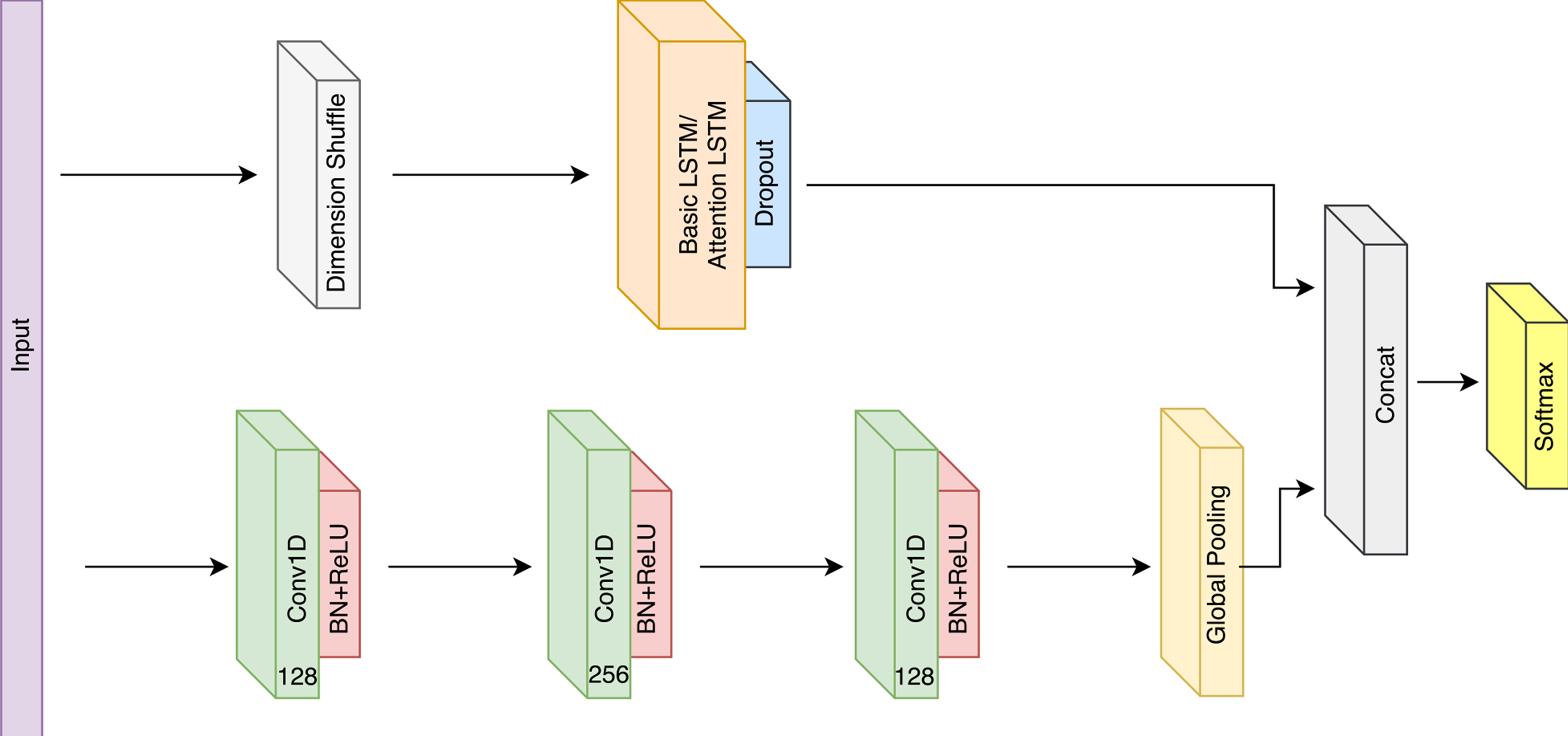
LSTM FCN models, from the paper LSTM Fully Convolutional Networks for Time Series Classification, augment the fast classification performance of Temporal Convolutional layers with the precise classification of Long Short Term Memory Recurrent Neural Networks.

Multivariate LSTM-FCN for Time Series Classification
General LSTM-FCNs are high performance models for univariate datasets. However, on multivariate datasets, we find that their performance is not optimal if applied directly. Therefore, we introduce Multivariate LSTM-FCN (MLSTM-FCN) for such datasets.
Paper: Multivariate LSTM-FCNs for Time Series Classification
Repository: MLSTM-FCN
Ablation Study of LSTM-FCN for Time Series Classification
Over the past year there have been several questions that have been raised by the community about the details of the model such as :
- Why we chose to augment a Fully Convolutional Network with an LSTM?
- What is dimension shuffle actually doing?
- After dimension shuffle, does the LSTM simply lose all recurrent behaviour?
- Why not replace the LSTM by another RNN such as GRU?
- Whether there is any actual improvement to be obtained from this augmentation?
We therefore perform a detailed ablation study, composing nearly 3,627 experiments that attempt to analyse and answer these questions and to provide a better understanding of the LSTM-FCN/ALSTM-FCN time series classification model and each of its sub-module.
The paper, titled Insights into LSTM Fully Convolutional Networks for Time Series Classification can be read for a thorough discussion and statistical analysis of the benefit of the Dimension Shuffled LSTM to the Fully Convolutional Network.
Paper: Insights into LSTM Fully Convolutional Networks for Time Series Classification Repository: LSTM-FCN-Ablation
Installation
Download the repository and apply pip install -r requirements.txt to install the required libraries.
Keras with the Tensorflow backend has been used for the development of the models, and there is currently no support for Theano or CNTK backends. The weights have not been tested with those backends.
The data can be obtained as a zip file from here - http://www.cs.ucr.edu/~eamonn/time_series_data/
Extract that into some folder and it will give 127 different folders. Copy paste the util script extract_all_datasets.py to this folder and run it to get a single folder _data with all 127 datasets extracted. Cut-paste these files into the Data directory.
Note : The input to the Input layer of all models will be pre-shuffled to be in the shape (Batchsize, 1, Number of timesteps), and the input will be shuffled again before being applied to the CNNs (to obtain the correct shape (Batchsize, Number of timesteps, 1)). This is in contrast to the paper where the input is of the shape (Batchsize, Number of timesteps, 1) and the shuffle operation is applied before the LSTM to obtain the input shape (Batchsize, 1, Number of timesteps). These operations are equivalent.
Training and Evaluation
All 127 UCR datasets can be evaluated with the provided code and weight files. Refer to the weights directory for clarification.
There is now exactly 1 script to run all combinations of the LSTM-FCN, and its Attention variant, on the three different Cell combinations (8, 64, 128), on all 127 datasets in a loop.
- To use the LSTM FCN model :
model = generate_lstmfcn() - To use the ALSTM FCN model :
model = generate_alstmfcn()
Training
Training now occurs in the innermost loop of the all_datasets_training.py.
A few parameters must be set in advance :
-
Datasets: Datasets must be listed as a pair (dataset name, id). The (name, id) pair for all 127 datasets has been preset. They correspond to the ids inside
constants.pyinside theutilsdirectory. ` -
Models : Models in the list must be defined as a (
model_name,model_function) pair. Please note : Themodel_functionmust be a model that returns a Keras Model, not an actual Model itself. Themodel_functioncan accept 3 parameters - maximum sequence length, number of classes and optionally the number of cells. -
Cells : The configurations of cells required to be trained over. The default is [8, 64, 128], corresponding to the paper.
After this, once training begins, each model will trained according to specificiation and log files will be written to which describe all the parameters for convenience along with the training and testing set accuracy at the end of training.
Weight files will automatically be saved in the correct directories and can be used for later analysis.
Training Inner-loop
To train the a model, uncomment the line below and execute the script. Note that '???????' will already be provided, so there is no need to replace it. It refers to the prefix of the saved weight file. Also, if weights are already provided, this operation will overwrite those weights.
train_model(model, did, dataset_name_, epochs=2000, batch_size=128,normalize_timeseries=normalize_dataset)
Evaluate Inner-loop
To evaluate the performance of the model, simply execute the script with the below line uncommented.
evaluate_model(model, did, dataset_name_, batch_size=128,normalize_timeseries=normalize_dataset)
Evaluate
There is no seperate script for evaluation. In order to re-evaluate trained models, please comment out the train_model function in the inner-most loop.
Visualization
Due to the automatic name generation of folders and weight paths, careful selection of 3 common parameters will be required for all of the visualizations below:
-
DATASET_ID: The unique integer id inside
constants.pyreferring to the dataset. -
num_cells: The number of LSTM / Attention LSTM Cells.
-
model: The model function used to build the corresponding Keras Model.
Next is the selection of the dataset_name and model_name. The dataset_name must match the name of the dataset inside the all_dataset_traning.py script. Similarly, the model_name must match the name of the model in MODELS inside all_dataset_training.py.
Filters Visualization
To visualize the output of the Convolution filters of either the LSTMFCN or the Attention LSTMFCN, utilize the visualize_filters.py script.
There are two parameters, CONV_ID which refers to the convolution block number (and therefore ranges from [0, 2]) and FILTER_ID whose value dictates which filters of the convolution layer is selected. Its range depends on the CONV_ID selected, rangeing from [0, 127] for CONV_ID = {0, 2} and [0, 255] for CONV_ID = 1.
Context Visualization
To visualize the context vector of the Attention LSTM module, please utilize the visualize_context.py script.
To generate the context over all samples in the dataset, modify LIMIT=None. Setting VISUALIZE_CLASSWISE=False is also recommended to speed up the computation. Note that for the larger datasets, generation of the image may take exorbitant amounts of time, and the output may not be pleasant. We suggest visualizing classwise with 1 sample per class instead, as shown above.
Class Activation Maps
To visualize the class activation map of the final convolution layer, execute the visualize_cam.py. The class of the input signal being visualized can be changed by changing the CLASS_ID from (0 to NumberOfClasses - 1).
Results
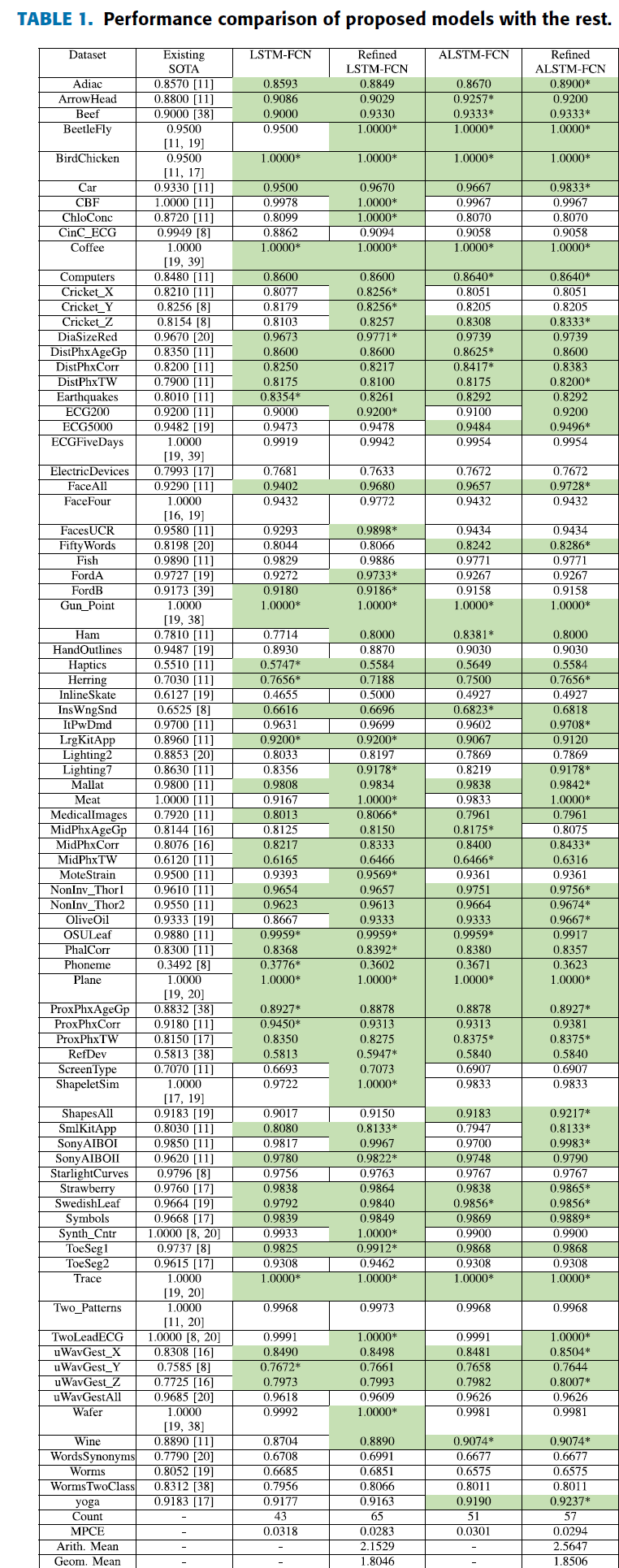
Results Based on Test Validation Checkpoint

Results Based on Minimum Training Loss

Critical Difference Diagram

Wilcoxson Signed Rank Test - Statistical Test
After applying a Dunn-Sidak Correction, we compare the p-value table to an alpha level of 0.00465. Results show ALSTM, LSTM, and the Ensemble Methods (COTE and EE) are statistically the same.

Citation
@article{karim2018lstm,
  title={LSTM fully convolutional networks for time series classification},
  author={Karim, Fazle and Majumdar, Somshubra and Darabi, Houshang and Chen, Shun},
  journal={IEEE Access},
  volume={6},
  pages={1662--1669},
  year={2018},
  publisher={IEEE}
}