GPAR

Implementation of the Gaussian Process Autoregressive Regression Model. See the paper, and see the docs.

• Requirements and Installation
• Basic Usage
• Features
  • Input and Output Dependencies
  • Output Transformation
  • Sampling
  • Logpdf Computation
  • Inducing Points
  • Example (examples/paper/synthetic.py)

Requirements and Installation

See the instructions here. Then simply

pip install gpar

Basic Usage

A simple instance of GPAR can be created as follows:

from gpar import GPARRegressor

gpar = GPARRegressor(
    replace=True,
    impute=True,
    scale=1.0,
    linear=True,
    linear_scale=100.0,
    nonlinear=True,
    nonlinear_scale=1.0,
    noise=0.1,
    normalise_y=True
)

Here the keyword arguments have the following meaning:

• replace=True: Replace data points with the posterior mean of the previous layer before feeding them into the next layer. This helps the model deal with noisy data, but may discard important structure in the data if the fit is bad.

• impute=True: GPAR requires that data is closed downwards. If this is not the case, the model will be unable to use part of the data. Setting impute to True lets GPAR impute data points to ensure that the data is closed downwards.

• scale=1.0: Initialisation of the length scale with respect to the inputs.

• linear=True: Use linear dependencies between outputs.

• linear_scale=100.0: Initialisation of the length scale of the linear dependencies between outputs.

• nonlinear=True: Also use nonlinear dependencies between outputs.

• nonlinear_scale=1.0: Initialisation of the length scale of the nonlinear dependencies between outputs. Important: this length scale applies after possible normalisation of the outputs (see below), in which case nonlinear_scale=1.0 corresponds to a simple, but nonlinear relationship.

• noise=0.1: Initialisation of the variance of the observation noise.

• normalise_y=True: Internally, work with a normalised version of the outputs by subtracting the mean and dividing by the standard deviation. Predictions will be transformed back appropriately.

In the above, any scalar hyperparameter may be replaced by a list of values to initialise each layer separately, e.g. scale=[1.0, 2.0]. See the documentation for a full overview of the keywords that may be passed to GPARRegressor.

By default, GPAR models dependencies between outputs as follows:

1. the first output y1 is modelled as a function of only the inputs x: y1 = y1(x);

2. the second output y2 is modelled as a function of the previous output y1 and the inputs x: y2 = y2(y1, x);

3. the third output y3 is modelled as a function of the previous outputs y2 and y1 and the inputs x: y3 = y3(y2, y1, x);

4. et cetera.

To fit GPAR, call gpar.fit(x_train, y_train) where x_train are the training inputs and y_train the training outputs. The inputs x_train must have shape (n,) or (n, m), where n is the number of data points and m the number of input features, and the outputs y_train must have shape (n,) or (n, p), where p is the number of outputs. Missing data can simply be set to np.nans. To condition GPAR on data without optimising its hyperparameters, use gpar.condition(x_train, y_train) instead.

Finally, to make predictions, call

means = gpar.predict(x_test, num_samples=100)

to get the predictive means, or

means, lowers, uppers = gpar.predict(
    x_test,
    num_samples=100, 
    credible_bounds=True
  )

to also get lower and upper 95% central marginal credible bounds. If you wish to predict the underlying latent function instead of the observed values, set latent=True in the call to GPARRegressor.predict.

Features

Input and Output Dependencies

Using keywords arguments, GPARRegressor can be configured to specify the dependencies with respect to the inputs and between the outputs. The following dependencies can be specified:

• Linear input dependencies: Set linear_input=True and specify the length scale with linear_input_scale.

• Nonlinear input dependencies: This is enabled by default. The length scale can be specified using scale. To tie these length scales across all layers, set scale_tie=True.

• Locally periodic input dependencies: Set per=True and specify the period with per_period, the length scale with per_scale, and the length scale on which the periodicity changes with per_decay.

• Linear output dependencies: Set linear=True and specify the length scale with linear_scale.

• Nonlinear output dependencies: Set nonlinear=True and specify the length scale with nonlinear_scale.

All nonlinear kernels are exponentiated quadratic kernels. If you wish to instead use rational quadratic kernels, set rq=True.

All parameters can be set to a list of values to initialise the value for each layer separately.

To let every layer depend only the kth previous layers, set markov=k.

Output Transformation

One may want to apply a transformation to the data before fitting the model, e.g. $y\mapsto\log(y)$ in the case of positive data. Such a transformation can be specified by setting the transform_y keyword argument for GPARRegressor. The following transformations are available:

• log_transform: $y \mapsto \log(y)$.

• squishing_transform: $y \mapsto \operatorname{sign}(y) \log(1 + |y|)$.

Sampling

Sampling from the model can be done with GPARRegressor.sample. The keyword argument num_samples specifies the number of samples, and latent specifies whether to sample from the underlying latent function or the observed values. Sampling from the prior and posterior (model must be fit first) can be done as follows:

sample = gpar.sample(x, p=2)  # Sample two outputs from the prior.

sample = gpar.sample(x, posterior=True)  # Sample from the posterior.

Logpdf Computation

The logpdf of data can be computed with GPARRegressor.logpdf. To compute the logpdf under the posterior, set posterior=True. To sample missing data to compute an unbiased estimate of the pdf, not logpdf, set sample_missing=True.

Inducing Points

Inducing points can be used to scale GPAR to large data sets. Simply set x_ind to the locations of the inducing points in GPARRegressor.

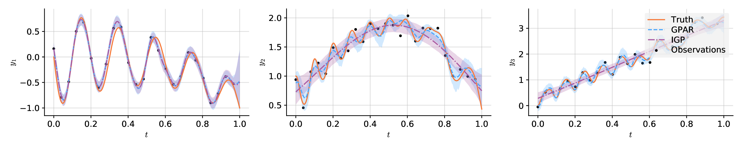
Example (examples/paper/synthetic.py)

import matplotlib.pyplot as plt
import numpy as np
from gpar.regression import GPARRegressor
from wbml.experiment import WorkingDirectory
import wbml.plot

if __name__ == "__main__":
    wd = WorkingDirectory("_experiments", "synthetic", seed=1)

    # Create toy data set.
    n = 200
    x = np.linspace(0, 1, n)
    noise = 0.1

    # Draw functions depending on each other in complicated ways.
    f1 = -np.sin(10 * np.pi * (x + 1)) / (2 * x + 1) - x ** 4
    f2 = np.cos(f1) ** 2 + np.sin(3 * x)
    f3 = f2 * f1 ** 2 + 3 * x
    f = np.stack((f1, f2, f3), axis=0).T

    # Add noise and subsample.
    y = f + noise * np.random.randn(n, 3)
    x_obs, y_obs = x[::8], y[::8]

    # Fit and predict GPAR.
    model = GPARRegressor(
        scale=0.1,
        linear=True,
        linear_scale=10.0,
        nonlinear=True,
        nonlinear_scale=0.1,
        noise=0.1,
        impute=True,
        replace=False,
        normalise_y=False,
    )
    model.fit(x_obs, y_obs)
    means, lowers, uppers = model.predict(
        x, num_samples=100, credible_bounds=True, latent=True
    )

    # Fit and predict independent GPs: set `markov=0` in GPAR.
    igp = GPARRegressor(
        scale=0.1,
        linear=True,
        linear_scale=10.0,
        nonlinear=True,
        nonlinear_scale=0.1,
        noise=0.1,
        markov=0,
        normalise_y=False,
    )
    igp.fit(x_obs, y_obs)
    igp_means, igp_lowers, igp_uppers = igp.predict(
        x, num_samples=100, credible_bounds=True, latent=True
    )

    # Plot the result.
    plt.figure(figsize=(15, 3))

    for i in range(3):
        plt.subplot(1, 3, i + 1)

        # Plot observations.
        plt.scatter(x_obs, y_obs[:, i], label="Observations", style="train")
        plt.plot(x, f[:, i], label="Truth", style="test")

        # Plot GPAR.
        plt.plot(x, means[:, i], label="GPAR", style="pred")
        plt.fill_between(x, lowers[:, i], uppers[:, i], style="pred")

        # Plot independent GPs.
        plt.plot(x, igp_means[:, i], label="IGP", style="pred2")
        plt.fill_between(x, igp_lowers[:, i], igp_uppers[:, i], style="pred2")

        plt.xlabel("$t$")
        plt.ylabel(f"$y_{i + 1}$")
        wbml.plot.tweak(legend=i == 2)

    plt.tight_layout()
    plt.savefig(wd.file("synthetic.pdf"))