SMART

SMART is a reference-free deconvolution method for spatial transcriptomics using marker-gene-assisted topic models.

Installation

You can install the development version of SMART from GitHub with:

# install.packages("devtools")
devtools::install_github("yyolanda/SMART")

Run SMART with example data

The base model of SMART takes the spatial transcriptomics data matrix (stData) and a list of marker gene symbols for each cell type (markerGs) as inputs.

The stData needs to be non-transformed counts (or round the data to the nearest integers).

Run the base model with:

library(SMART)
data(visium_mouse_brain)
base_res <- SMART_base(stData=visium_mouse_brain$stMat,
                       markerGs=visium_mouse_brain$markers, 
                       noMarkerCts=1,outDir='SMART_results',seed=8001)

To make a scatterpie plot showing the predicted proportions for all cell types:

SMART_scatterpie(visium_mouse_brain$loc,res$ct_proportions)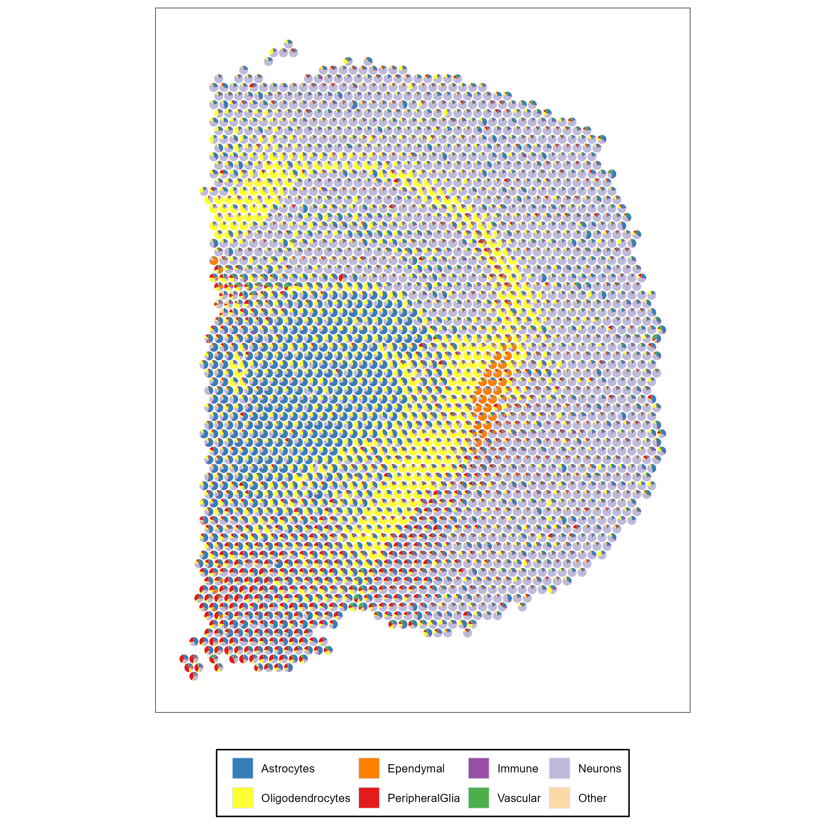

To make a scatterheatmap showing the predicted proportions for a selected cell type:

SMART_scatterheatmap(visium_mouse_brain$loc,res$ct_proportions, celltype = 'Oligos')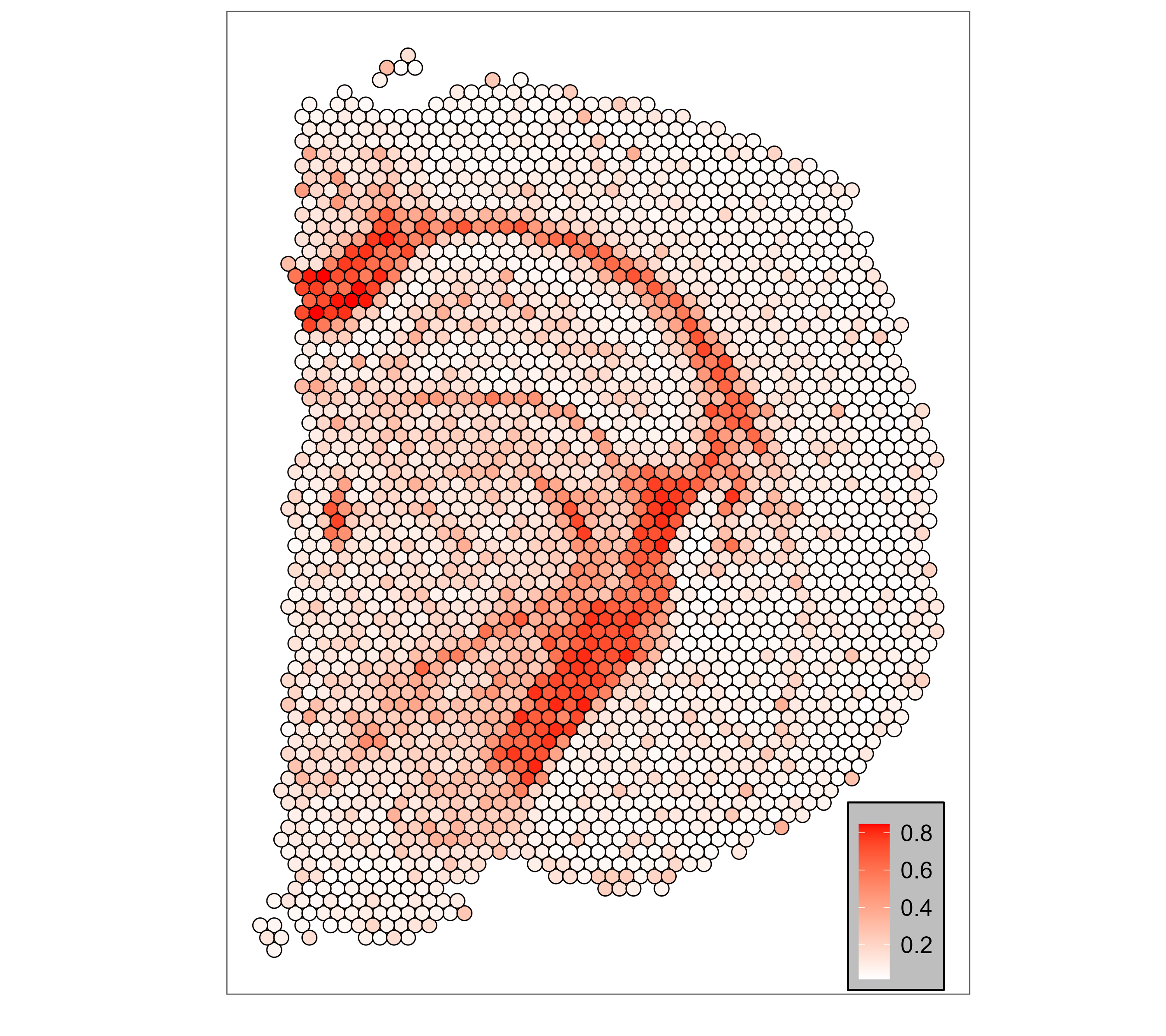

You may also obtain more stable cell type composition by running multiple instances of SMART and averaging the results.

# the number of instances
mc.cores=10

# the output directory
out.dir='SMART_results/testrun/'

# set random starting values
set.seed(1)
seeds=sample(1:1000000,mc.cores,replace = FALSE)

# for windows
library(future)
library(future.apply)
plan(future.callr::callr,workers=mc.cores)
res=future_lapply(seeds,
  FUN = function(x) SMART_base(stData=visium_mouse_brain$stMat,
                              markerGs=visium_mouse_brain$markers, 
                              noMarkerCts=1, outDir=out.dir,
                              seed=x),
  future.stdout = TRUE,future.seed = NULL)

tmp=lapply(res, function(x) x$ct_proportions/rowSums(x$ct_proportions))
tmp2=Reduce('+', tmp)
res_avg=tmp2/rowSums(tmp2)

# for linux, you may also use
library(doMC)
doMC::registerDoMC(cores=mc.cores)
foreach(i = seeds) %dopar% {
  res <- SMART_base(stData=visium_mouse_brain$stMat, 
                    markerGs=visium_mouse_brain$markers, 
                    noMarkerCts=1, 
                    outDir=out.dir, 
                    seed=i)
} 
res=lapply(seeds,function(x) readRDS(paste0('SMART_results/testrun/inst_',x,'/base_model.rds')))
tmp=lapply(res, function(x) x$theta/rowSums(x$theta))
tmp2=Reduce('+', tmp)
res_avg=tmp2/rowSums(tmp2)

Consider running it serially if there is not enough RAM. Running it in parallel also disables the progressing bar.

Run the covariate model with example data

The covariate model of SMART takes the spatial transcriptomics data matrix (stData), a list of marker gene symbols for each cell type (markerGs), a data.frame of covariate levels (covarDat) and the covariates (covars) as inputs.

Run the covariate model with:

data(MPOA)
mod <- SMART_covariate(stData=MPOA$stMat, markerGs=MPOA$markers,       
                       covarDat=MPOA$covDat,covars='sex',
                       noMarkerCts=1,outDir='SMART_results', seed=1)
cov_res <- get_est(model=mod$model, stData=MPOA$stMat, 
                   covarDat=MPOA$covDat, covar='sex')

Then, we can compute the log2 fold change between the conditions (Female vs. Male).

geneList=log2(cov_res$ct_spec_gexp$F$phi/cov_res$ct_spec_gexp$M$phi)['Inhibitory',] %>% sort()

Next, we perform a gene set enrichment analysis for each cell type. Here we use the "fgsea" R package to obtain the GO biological processes, GO molecular functions, and Reactome pathways associated with sex. The .gmt files can be downloaded from MSigDB (https://www.gsea-msigdb.org/gsea/msigdb/index.jsp).

library(fgsea)
gseaRes=list()
for(gmt in c('m5.go.bp.v2023.1.Mm.symbols.gmt','m5.go.mf.v2023.1.Mm.symbols.gmt',
             'm2.cp.reactome.v2023.1.Mm.symbols.gmt')){
        print(gmt)
        pathways <- gmtPathways(paste0('GSEA/',gmt))
        fgseaRes <- fgsea(pathways = pathways,
                        stats    = geneList,
                        minSize  = 10,
                        maxSize  = 1000,
                        nperm=1000)
        gseaRes[[gmt]]=fgseaRes %>% filter(padj<0.1) %>% arrange(pval) %>% mutate(database=gmt)
}   
gseaRes=rbindlist(gseaRes)

Run the two-stage model with example data

The two-stage model of SMART takes the spatial transcriptomics data matrix (stData), a list of marker gene symbols to be used to deconvolve cell types into major cell types (markers_S1), a list of marker gene symbols to be used to deconvolve the cell type of interest into its subtypes (markers_S2), the cell type of interest (CT_OI), the cell type that is transcriptomically similar to the cell type of interest (CT_similar) as inputs.

The CT_similar can be NULL, a character value specifying a cell type name, or 'auto' to automatically select the most similar cell type.

Run the two-stage model with:

data(NSCLC)
TS_res <- SMART_2S(NSCLC$stData, NSCLC$markers_S1, NSCLC$markers_S2,
                   noMarkerCts_S1=1, noMarkerCts_S2=1,
                   CT_OI='DC',CT_similar='macrophage',
                   outDir='SMART_results')

The resulting object contains the models from each of the two stages as well as the final cell type proportions of each spot.