meshpro/optimesh - Githubissues

Triangular mesh optimization.

Several mesh smoothing/optimization methods with one simple interface. optimesh

is fast,
preserves submeshes,
only works for triangular meshes, flat and on a surface, (for now; upvote this issue if you're interested in tetrahedral mesh smoothing), and
supports all mesh formats that meshio can handle.

Installation

Install optimesh from PyPI with

pip install optimesh

How to get a license

Licenses for personal and academic use can be purchased here. You'll receive a confirmation email with a license key. Install the key with

slim install <your-license-key>

on your machine and you're good to go.

For commercial use, please contact support@mondaytech.com.

Using optimesh

Example call:

optimesh in.e out.vtk

Output: terminal-screenshot

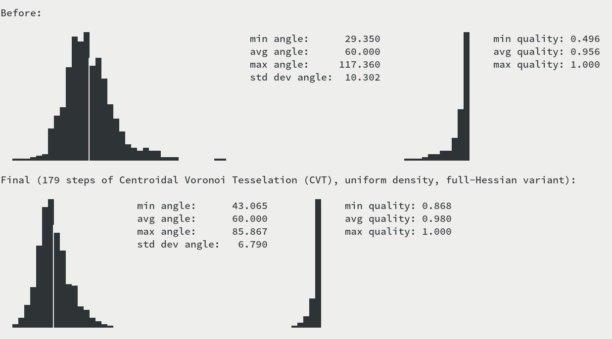
The left hand-side graph shows the distribution of angles (the grid line is at the optimal 60 degrees). The right hand-side graph shows the distribution of simplex quality, where quality is twice the ratio of circumcircle and incircle radius.

All command-line options are documented at

optimesh -h

Showcase

disk-step0

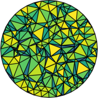
The following examples show the various algorithms at work, all starting from the same randomly generated disk mesh above. The cell coloring indicates quality; dark green is bad, yellow is good.

CVT (centroidal Voronoi tessellation)


uniform-density relaxed Lloyd's algorithm (`--method lloyd --omega 2.0`)	uniform-density quasi-Newton iteration (block-diagonal Hessian, `--method cvt-block-diagonal`)	uniform-density quasi-Newton iteration (default method, full Hessian, `--method cvt-full`)

Centroidal Voronoi tessellation smoothing (Du et al.) is one of the oldest and most reliable approaches. optimesh provides classical Lloyd smoothing as well as several variants that result in better meshes.

CPT (centroidal patch tessellation)


density-preserving linear solve (Laplacian smoothing, `--method cpt-linear-solve`)	uniform-density fixed-point iteration (`--method cpt-fixed-point`)	uniform-density quasi-Newton (`--method cpt-quasi-newton`)

A smoothing method suggested by Chen and Holst, mimicking CVT but much more easily implemented. The density-preserving variant leads to the exact same equation system as Laplacian smoothing, so CPT smoothing can be thought of as a generalization.

The uniform-density variants are implemented classically as a fixed-point iteration and as a quasi-Newton method. The latter typically converges faster.

ODT (optimal Delaunay tessellation)


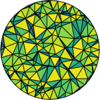
density-preserving fixed-point iteration (`--method odt-dp-fp`)	uniform-density fixed-point iteration (`--method odt-fixed-point`)	uniform-density BFGS (`--method odt-bfgs`)

Optimal Delaunay Triangulation (ODT) as suggested by Chen and Holst. Typically superior to CPT, but also more expensive to compute.

Implemented once classically as a fixed-point iteration, once as a nonlinear optimization method. The latter typically leads to better results.

Using optimesh from Python

You can also use optimesh in a Python program. Try

import optimesh

# [...] create points, cells [...]

points, cells = optimesh.optimize_points_cells(
    points, cells, "CVT (block-diagonal)", 1.0e-5, 100
)

# or create a meshplex Mesh
import meshplex

mesh = meshplex.MeshTri(points, cells)
optimesh.optimize(mesh, "CVT (block-diagonal)", 1.0e-5, 100)
# mesh.points, mesh.cells, ...

If you only want to do one optimization step, do

points = optimesh.get_new_points(mesh, "CVT (block-diagonal)")

Surface mesh smoothing

optimesh also supports optimization of triangular meshes on surfaces which are defined implicitly by a level set function (e.g., spheres). You'll need to specify the function and its gradient, so you'll have to do it in Python:

import meshzoo
import optimesh

points, cells = meshzoo.tetra_sphere(20)

class Sphere:
    def f(self, x):
        return 1.0 - (x[0] ** 2 + x[1] ** 2 + x[2] ** 2)

    def grad(self, x):
        return -2 * x

# You can use all methods in optimesh:
points, cells = optimesh.optimize_points_cells(
    points,
    cells,
    "CVT (full)",
    1.0e-2,
    100,
    verbose=False,
    implicit_surface=Sphere(),
    # step_filename_format="out{:03d}.vtk"
)

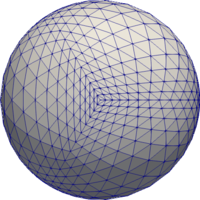
This code first generates a mediocre mesh on a sphere using meshzoo,

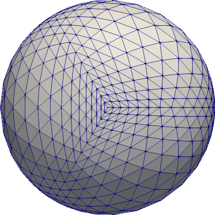
and then optimizes. Some results:


CPT	ODT	CVT (full Hessian)

Which method is best?

From practical experiments, it seems that the CVT smoothing variants, e.g.,

optimesh in.vtk out.vtk -m cvt-uniform-qnf

give very satisfactory results. (This is also the default method, so you don't need to specify it explicitly.) Here is a comparison of all uniform-density methods applied to the random circle mesh seen above:

(Mesh quality is twice the ratio of incircle and circumcircle radius, with the maximum being 1.)

Why optimize?


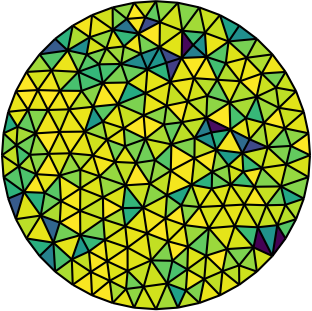
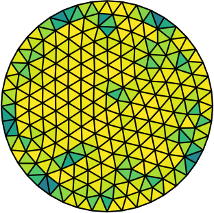
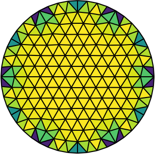
Gmsh mesh	Gmsh mesh after optimesh	dmsh mesh

Let us compare the properties of the Poisson problem (Δu = f with Dirichlet boundary conditions) when solved on different meshes of the unit circle. The first mesh is the on generated by Gmsh, the second the same mesh but optimized with optimesh, the third a very high-quality dmsh mesh.

We consider meshings of the circle with an increasing number of points:


average cell quality	condition number of the Poisson matrix	number of CG steps for Poisson problem

Quite clearly, the dmsh generator produces the highest-quality meshes (left). The condition number of the corresponding Poisson matrices is lowest for the high quality meshes (middle); one would hence suspect faster convergence with Krylov methods. Indeed, most CG iterations are necessary on the Gmsh mesh (right). After optimesh, one saves between 10 and 20 percent of iterations/computing time. The dmsh mesh cuts the number of iterations in half.

Access from Python

All optimesh functions can also be accessed from Python directly, for example:

import optimesh

X, cells = optimesh.odt.fixed_point(X, cells, 1.0e-2, 100, verbose=False)