![]()
3D Data Cube Visualization in Jupyter Notebooks
GitHub: https://github.com/msoechting/lexcube
Paper: https://doi.org/10.1109/MCG.2023.3321989
PyPI: https://pypi.org/project/lexcube/
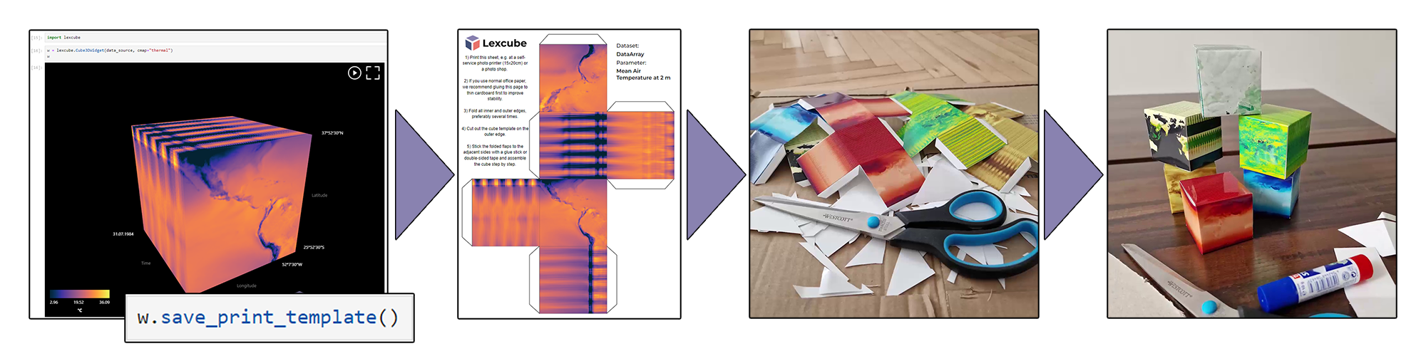
NEW with version 0.4.16: Craft your own paper data cube!
Lexcube is a library for interactively visualizing three-dimensional floating-point data as 3D cubes in Jupyter notebooks.
Supported data formats:
- numpy.ndarray (with exactly 3 dimensions)
- xarray.DataArray (with exactly 3 dimensions, rectangularly gridded)
Possible data sources:
- Any gridded Zarr or NetCDF data set (local or remote, e.g., accessed with S3)
- Copernicus Data Storage, e.g., ERA5 data
- Google Earth Engine (using xee, see example notebook)
Example notebooks can be found in the examples folder. For a live demo, see also lexcube.org.
Table of Contents
- Attribution
- How to Use Lexcube
- Installation
- Cube Visualization
- Interacting with the Cube
- Range Boundaries
- Colormaps
- Save figures
- Print your own paper data cube
- Supported metadata
- Troubleshooting
- The cube does not respond / API methods are not doing anything / Cube does not load new data
- After installation/update, no widget is shown, only text
- w.savefig breaks when batch-processing/trying to create many figures quickly
- The layout of the widget looks very messed up
- "Error creating WebGL context" or similar
- Memory is filling up a lot when using a chunked dataset
- Known bugs
- Attributions
- Development Installation \& Guide
- License
Attribution
When using Lexcube and/or generated images, please acknowledge/cite:
@ARTICLE{soechting2024lexcube,
  author={Söchting, Maximilian and Mahecha, Miguel D. and Montero, David and Scheuermann, Gerik},
  journal={IEEE Computer Graphics and Applications},
  title={Lexcube: Interactive Visualization of Large Earth System Data Cubes},
  year={2024},
  volume={44},
  number={1},
  pages={25-37},
  doi={10.1109/MCG.2023.3321989}
}
Lexcube is a project by Maximilian Söchting at the RSC4Earth at Leipzig University, advised by Prof. Dr. Miguel D. Mahecha and Prof. Dr. Gerik Scheuermann. Thanks to the funding provided by ESA through DeepESDL and DFG through the NFDI4Earth pilot projects!
How to Use Lexcube
Example Notebooks
If you are new to Lexcube, try the general introduction notebook which demonstrates how to visualize a remote Xarray data set.
There are also specific example notebooks for the following use cases:
- Visualizing Google Earth Engine data - using xee
- Generating and visualizing a spectral index data cube from scratch - using cubo and spyndex, with data from Microsoft Planetary Computer
- Generating and visualizing a spectral index data cube - with data from OpenEO
- Visualizing Numpy data
Minimal Examples for Getting Started
Visualizing Xarray Data
import xarray as xr
import lexcube
ds = xr.open_dataset("http://data.rsc4earth.de/EarthSystemDataCube/v3.0.2/esdc-8d-0.25deg-256x128x128-3.0.2.zarr/", chunks={}, engine="zarr")
da = ds["air_temperature_2m"][256:512,256:512,256:512]
w = lexcube.Cube3DWidget(da, cmap="thermal_r", vmin=-20, vmax=30)
w
Visualizing Numpy Data
import numpy as np
import lexcube
data_source = np.sum(np.mgrid[0:256,0:256,0:256], axis=0)
w = lexcube.Cube3DWidget(data_source, cmap="prism", vmin=0, vmax=768)
w
Visualizing Google Earth Engine Data
import lexcube
import xarray as xr
import ee
ee.Authenticate()
ee.Initialize(opt_url="https://earthengine-highvolume.googleapis.com")
ds = xr.open_dataset("ee://ECMWF/ERA5_LAND/HOURLY", engine="ee", crs="EPSG:4326", scale=0.25, chunks={})
da = ds["temperature_2m"][630000:630003,2:1438,2:718]
w = lexcube.Cube3DWidget(da)
w
Note on Google Collab
If you are using Google collab, you may need to execute the following before running Lexcube:
from google.colab import output
output.enable_custom_widget_manager()
Note on Juypter for VSCode
If you are using Jupyter within VSCode, you may have to add the following to your settings before running Lexcube:
    "jupyter.widgetScriptSources": [
        "jsdelivr.com",
        "unpkg.com"
    ],
If you are working on a remote server in VSCode, do not forget to set this setting also there! This allows the Lexcube JavaScript front-end files to be downloaded from these sources (read more).
Installation
You can install using pip:
pip install lexcubeAfter installing or upgrading Lexcube, you should refresh the Juypter web page (if currently open) and restart the kernel (if currently running).
If you are using Jupyter Notebook 5.2 or earlier, you may also need to enable the nbextension:
jupyter nbextension enable --py [--sys-prefix|--user|--system] lexcubeCube Visualization
On the cube, the dimensions are visualized as follow: X from left-to-right (0 to max), Y from top-to-bottom (0 to max), Z from back-to-front (0 to max); with Z being the first dimension (axis[0]), Y the second dimension (axis[1]) and X the third dimension (axis[2]) on the input data. If you prefer to flip any dimension or re-order dimensions, you can modify your data set accordingly before calling the Lexcube widget, e.g. re-ordering dimensions with xarray: ds.transpose(ds.dims[0], ds.dims[2], ds.dims[1]) and flipping dimensions with numpy: np.flip(ds, axis=1).
Interacting with the Cube
- Zooming in/out on any side of the cube:
- Mousewheel
- Scroll gesture on touchpad (two fingers up or down)
- On touch devices: Two-touch pinch gesture
- Panning the currently visible selection:
- Click and drag the mouse cursor
- On touch devices: touch and drag
- Moving over the cube with your cursor will show a tooltip in the bottom left about the pixel under the cursor.
- For more precise input, you can use the sliders provided by
w.show_sliders():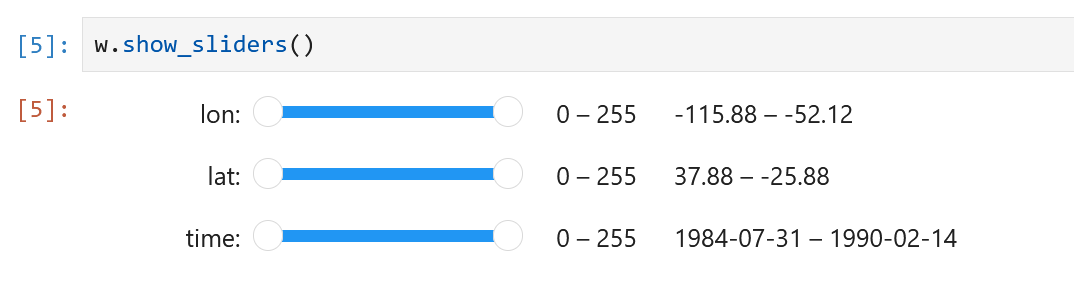
Range Boundaries
You can read and write the boundaries of the current selection via the xlim, ylim and zlim tuples.
w = lexcube.Cube3DWidget(da, cmap="thermal", vmin=-20, vmax=30)
w
# Next cell:
w.xlim = (20, 400)
For fine-grained interactive controls, you can display a set of sliders in another cell, like this:
w = lexcube.Cube3DWidget(da, cmap="thermal", vmin=-20, vmax=30)
w
# Next cell:
w.show_sliders()
For very large data sets, you may want to use w.show_sliders(continuous_update=False) to prevent any data being loaded before making a final slider selection.
If you want to wrap around a dimension, i.e., seamleasly scroll over back to the 0-index beyond the maximum index, you can enable that feature like this:
w.xwrap = TrueFor data sets that have longitude values in their metadata very close to a global round-trip, this is automatically active for the X dimension.
Limitations: Currently only supported for the X dimension. If xwrap is active, the xlim tuple may contain values up to double the valid range to always have a range where x_min < x_max. To get values in the original/expected range, you can simply calculate x % x_max.
Colormaps
All colormaps of matplotlib and cmocean are supported.
The range of the colormap, if not set using vmin/vmax, is automatically adjusted to the approximate observed minimum and maximum valuesnote within the current session. Appending "_r" to any colormap name will reverse it.
# 1) Set cmap in constructor
w = lexcube.Cube3DWidget(da, cmap="thermal", vmin=-20, vmax=30)
w

# 2) Set cmap later
w.cmap = "thermal"
w.vmin = -20
w.vmax = 30

# 3) Set custom colormap using lists (evenly spaced RGB values)
w.cmap = cmocean.cm.thermal(np.linspace(0.0, 1.0, 100)).tolist()
w.cmap = [[0.0, 0.0, 0.0], [1.0, 0.5, 0.5], [0.5, 1.0, 1.0]]
note Lexcube actually calculates the mean of all values that have been visible so far in this session and applies ±2.5σ (standard deviation) in both directions to obtain the colormap ranges, covering approximately 98.7% of data points. This basic method allows to filter most outliers that would otherwise make the colormap range unnecessarily large and, therefore, the visualization uninterpretable.
Supported colormaps
Cmocean:
- "thermal", "haline", "solar", "ice", "gray", "oxy", "deep", "dense", "algae", "matter", "turbid", "speed", "amp", "tempo", "rain", "phase", "topo", "balance", "delta", "curl", "diff", "tarn"
Proplot custom colormaps:
- "Glacial", "Fire", "Dusk", "DryWet", "Div", "Boreal", "Sunset", "Sunrise", "Stellar", "NegPos", "Marine"
Scientific Colormaps by Crameri:
- "acton", "bam", "bamako", "bamO", "batlow", "batlowK", "batlowW", "berlin", "bilbao", "broc", "brocO", "buda", "bukavu", "cork", "corkO", "davos", "devon", "fes", "glasgow", "grayC", "hawaii", "imola", "lajolla", "lapaz", "lisbon", "lipari", "managua", "navia", "nuuk", "oleron", "oslo", "roma", "romaO", "tofino", "tokyo", "turku", "vanimo", "vik", "vikO"
PerceptuallyUniformSequential:
- "viridis", "plasma", "inferno", "magma", "cividis"
Sequential:
- "Greys", "Purples", "Blues", "Greens", "Oranges", "Reds", "YlOrBr", "YlOrRd", "OrRd", "PuRd", "RdPu", "BuPu", "GnBu", "PuBu", "YlGnBu", "PuBuGn", "BuGn", "YlGn"
Sequential(2):
- "binary", "gist_yarg", "gist_gray", "gray", "bone", "pink", "spring", "summer", "autumn", "winter", "cool", "Wistia", "hot", "afmhot", "gist_heat", "copper"
Diverging:
- "PiYG", "PRGn", "BrBG", "PuOr", "RdGy", "RdBu", "RdYlBu", "RdYlGn", "Spectral", "coolwarm", "bwr", "seismic",
Cyclic:
- "twilight", "twilight_shifted", "hsv"
Qualitative:
- "Pastel1", "Pastel2", "Paired", "Accent", "Dark2", "Set1", "Set2", "Set3", "tab10", "tab20", "tab20b", "tab20c"
Miscellaneous:
- "flag", "prism", "ocean", "gist_earth", "terrain", "gist_stern", "gnuplot", "gnuplot2", "CMRmap", "cubehelix", "brg", "gist_rainbow", "rainbow", "jet", "nipy_spectral", "gist_ncar"
Save figures
You can save PNG images of the cube like this:
w.savefig(fname="cube.png", include_ui=True, dpi_scale=2.0)fname: name of the image file. Default:lexcube-{current time and date}.png.include_ui: whether to include UI elements such as the axis descriptions and the colormap legend in the image. Default:true.dpi_scale: the image resolution is multiplied by this value to obtain higher-resolution/quality images. For example, a value of 2.0 means that the image resolution is doubled for the PNG vs. what is visible in the notebook. Default:2.0.
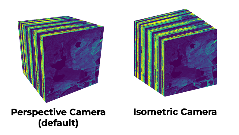
If you want to edit multiple cubes into one picture, you may prefer an isometric rendering. You can enable it in the constructor: lexcube.Cube3DWidget(data_source, isometric_mode=True). For comparison:
Print your own paper data cube
You can generate a template to make your own paper data cube from your currently visible data cube like this:
w.save_print_template()In the opened dialog, you can download the print template as either PNG or SVG to your computer. You can also add a custom note to the print template, e.g. to remember specifics about the data set. Printing (recommended: thick paper or photo paper, e.g. 15x20cm), cutting and gluing will give you your own paper data cube for your desk:
Supported metadata
When using Xarray for the input data, the following metadata is automatically integrated into the visualization:
- Dimension names
- Read from the xarray.DataArray.dims attribute
- Parameter name
- Read from the xarray.DataArray.attrs.long_name attribute
- Units
- Read from the xarray.DataArray.attrs.units attribute
- Indices
- Time indices are converted to UTC and displayed in local time in the widget
- Latitude and longitude indices are displayed in their full forms in the widget
- Other indices (strings, numbers) are displayed in their full form
- If no indices are available, the numeric indices are displayed
Troubleshooting
Below you can find a number of different common issues when working with Lexcube. If the suggested solutions do not work for you, feel free to open an issue!
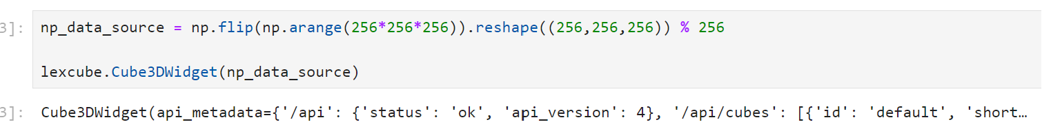
The cube does not respond / API methods are not doing anything / Cube does not load new data
Under certain circumstances, the widget may get disconnected from the kernel. You can recognize it with this symbol (crossed out chain 🔗):
Possible Solutions:
- Execute the cell again
- Restart the kernel
- Refresh the web page (also try a "hard refresh" using CTRL+F5 or Command+Option+R - this forces the browser to ignore its cache)
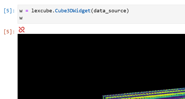
After installation/update, no widget is shown, only text
Example:
Possible solutions:
- Restart the kernel
- Refresh the web page (also try a "hard refresh" using CTRL+F5 or Command+Option+R - this forces the browser to ignore its cache)
w.savefig breaks when batch-processing/trying to create many figures quickly
The current savefig implementation is limited by its asynchronous nature. This means that the savefig call returns before the image is rendered and downloaded. Therefore, a workaround, such as waiting one second between images, is necessary to correctly create images when batchprocessing.
The layout of the widget looks very messed up
This can happen in old versions of browsers. Update your browser or use a modern, up-to-date browser such as Firefox or Chrome. Otherwise, feel free to create an issue with your exact specs.
"Error creating WebGL context" or similar
WebGL 2 seems to be not available or disabled in your browser. Check this page to test if your browser is compatible: https://webglreport.com/?v=2. Possible solutions are:
- Update your browser
- Update your video card drivers
Memory is filling up a lot when using a chunked dataset
Lexcube employs an alternative, more aggressive chunk caching mechanism in contrast to xarray. It will cache any touched chunk in memory without releasing it until the widget is closed. Disabling it will most likely decrease memory usage but increase the average data access latency, i.e., make Lexcube slower. To disable it, use: lexcube.Cube3DWidget(data_source, use_lexcube_chunk_caching=False).
Known bugs
- Zoom interactions with the mousewheel may be difficult for data sets with very small ranges on some dimensions (e.g. 2-5).
- Zoom interactions may behave unexpectedly when zooming on multiple cube faces subsequently.
Attributions
Lexcube uses lots of amazing open-source software and packages, including:
- Data access: Xarray & Numpy
- Lossy floating-point compression: ZFP
- Client boilerplate: TypeScript Three.js Boilerplate by Sean Bradley
- Jupyter widget boilerplate: widget-ts-cookiecutter
- Colormaps: matplotlib, cmocean, Scientific colour maps by Fabio Crameri, Proplot custom colormaps
- 3D graphics engine: Three.js (including the OrbitControls, which have been modified for this project)
- Client bundling: Webpack
- UI sliders: Nouislider
- Decompression using WebAssembly: numcodecs.js
- WebSocket communication: Socket.io
Development Installation & Guide
See CONTRIBUTING.md.
License
The Lexcube application core, the Lexcube Jupyter extension, and other portions of the official Lexcube distribution not explicitly licensed otherwise, are licensed under the GNU GENERAL PUBLIC LICENSE v3 or later (GPLv3+) -- see the "COPYING" file in this directory for details.