Requirement: This repository is included in the official release of FragM. You can run the examples by installing FragM and navigating to examples >> neozhaoliang.

In this project, We will visualize hyperbolic Coxeter groups of varying ranks 3/4/5 and levels 1/2/3. The scenes can be categorized into two types:

1. Tiling display: Show the tiling of hyperbolic honeycombs inside the space in the Poincaré ball and upper half-space models.
2. Sphere packing display: Show the sphere packing on the ideal boundary. The complement of this sphere packing is called the limit set.

The level of a Coxeter group $G$ is defined as the smallest non-negative integer $l$, such that after removing any $l$ vertices from its Coxeter diagram, all connected components of the remaining diagram are finite or affine. For example, finite (spherical) and affine (Euclidean) Coxeter groups have level 0.

It's proved in a paper by George Maxwell that Coxeter groups of level 1 or 2 are both hyperbolic. For level 1, the limit set is the ideal boundary and there is no sphere packing. For level 2, there is a maximal sphere packing on the ideal boundary, meaning the spheres do not intersect and fill the boundary. For levels higher than 2, the spheres still fill the boundary, but they will overlap. For further mathematical details, please refer to the paper by Chen and Labbé (Chen and Labbé's paper) on the connection between hyperbolic geometry and sphere packings.

3D Euclidean tilings (rank = 4, level = 0)

Shadertoy live

2D hyperbolic tilings (rank = 3, level = 1, 2)

Shadertoy live

From left to right: compact tiling, paracompact tiling (with ideal vertices on the boundary), non-compact tiling (with hyperideal vertices outside the space)

The level 2 case in the rightmost image appears less attractive. However, it can be observed that each cell, which is an unbounded triangle, intersects the ideal boundary at an arc. All these arcs pack the entire boundary circle. This phenomenon generalizes to three and four-dimensional spaces. If the group has level 2, each cell in the honeycomb will intersect the boundary at a disk/sphere, and these disks/spheres pack the entire boundary.

3D hyperbolic honeycombs (rank = 4, level = 1, 2)

The code used to render the following image is here. It can render any hyperbolic group of rank 4 that has all labels $m_{s,t}<\infty$ and contains a finite sub-diagram of rank 3. (Images with Poincaré disks packing the boundary are of level 2)

2D circle packings (rank = 4, level = 2)

Shadertoy live

2D circles packings (rank = 4, level > 2)

In this case, there will be overlapping circles:

Circle packings from platonic solids

In order (left to right, top to bottom): tetrahedron, cube, octahedron, dodecahedron, icosahedron.

Shadertoy Live

Non-reflective circle packings

These packings follow from a preprint of Kapovich and Kontorovich. Level not defined.

Extended Bianchi groups. Left: Bi23. Right: Bi31.

Groups from Mcleod's thesis. Left: Modified f(3,6). Right: f(3,14).

2D slices of 3D ball packings (rank = 5, level = 2)

Shadertoy live

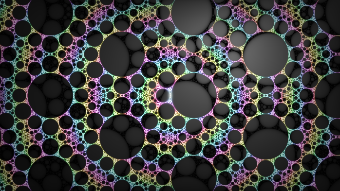
3D ball packings (rank = 5, level >= 2)

These are the ball packings in the next section but shown in the Poincaré unit ball model.

Fractals from 3D ball clusters (rank = 5, level = 3)

How to use this project in FragM

Please refer to the official Wiki page of FragM for more detailed information on how to use it.

• Download or clone this repository to your local machine.

• Visit the Fragmentarium release page and select the appropriate release for your operating system. In this tutorial, the instructions are based on a Windows environment. Therefore, download the file Fragmentarium-2.5.7-221224-winex.7z. Save the file and extract it to a convenient location on your disk.

  

• In the extracted folder, locate the executable file named Fragmentarium-2.5.7.exe. Double-click it to launch the application. Upon launching, you should see the following interface:

  

  The interface is organized into four main regions:

  1. The central area displays the rendered result based on the loaded .frag file.
  2. On the left side, you will find the code editor. If you make changes to the source code, press Ctrl + S to save your modifications, then click Build to recompile and view the updated result.
  3. The right side houses the control panel, where you can adjust various parameters. These controls are defined within the .frag file using #group macros.
  4. The bottom section is dedicated to logging. If the code fails to compile, check the error messages here for troubleshooting information.

• From the menu bar, select File -> Open. Navigate to the directory where you saved the source code of this project and choose a .frag file. For example, select Ball-Packings-UHS.frag. Fragmentarium will load and compile the file, displaying the rendered output on your screen:

  

Authors

• Chen Hao
• Zhao Liang
• Abdelaziz Nait Merzouk

License

The .frag code written for FragM in this repository is licensed under the GPL License. The images demonstrated by the authors in this project, including those uploaded by the authors on other platforms such as Twitter, are licensed under the CC BY-NC-SA license.