
NanoBlot: An R Package for Visualization of RNA Isoforms from Long Read RNA-sequencing Data
RT-PCR and northern blots have long been used to study RNA isoforms usage for single genes. Recently, advancements in long read sequencing have yielded unprecedented information about the usage and abundance of these RNA isoforms. However, visualization of long-read sequencing data remains challenging due to the high information density. To alleviate these issues we have developed NanoBlot, an open-source, R-package, which generates northern blot and RT-PCR-like images from long-read sequencing data. NanoBlot requires aligned, positionally sorted and indexed BAM files. Plotting is based around ggplot2 and is easily customizable. Advantages of nanoblots include: A robust system for designing probes to visualize isoforms including excluding reads based on the presence or absence of a specified region, an elegent solution to representing isoforms with continuous variations in length, and the ability to overlay multiple genes in the same plot using different colors. We present examples of nanoblots compared to actual northern blot data. In addition to traditional gel-like images, the NanoBlot package can also output other visualizations such as violin plots and 3′-RACE-like plots focused on 3′-ends isoforms visualization. The use of the NanoBlot package should provide a simple answer to some of the challenges of visualizing long-read RNA sequencing data.
Basic Usage
The NanoBlot R package can be loaded entirely using the devtools package built into R. First, make sure that you have the devtools package in R.
install.packages("devtools")
Then, make sure you are in the right directory for the R NanoBlot package folder, which should end in something like "/NanoBlotPackage". Then, run this code to compile NanoBlot
devtools::install(build_vignettes = TRUE)
If there are any build errors, the most common reason is the conda environment is not set up. Please reference below
After installing, you can load the package using a simple library command
library("NanoBlotPackage")
NanoBlot is now ready for use!
Setting up conda environment
Some core NanoBlot functions will rely on system() commands that are expected to be built into the user's console. These commands include packages like bedtools and samtools as there is no R equivalent that works as efficiently. Thus, if the user does not have previous path commands in their console environment, the user can utilize the prewritten conda environment for easy installation. The provided conda .yml environment is listed under the scripts folder and titled nanoblotenv.yml
The steps to install the conda environment are as followed
Step 1: Install anaconda if not already on computer. Then find the system path to conda using the command which conda in any terminal of your choice.
Step 2: Call the function conda create -f {your path}/scripts/nanoblotenv.yml in either the terminal, or you can call it in R using the function
system2("{your path to conda}, args = c("env", "create", "-f", "{your path}/scripts/nanoblotenv.yml"))
Step 3: Add the newly created environment into R's system path so that R will automatically search for it using this code block
old_path <- Sys.getenv("PATH")
Sys.setenv(PATH = paste(old_path, "{path to conda environment}", sep = ":"))
Basic Workflow

Code Example
We start by subsetting our example data files to the probe RPL18A Note that we store this in a specified temp folder. If a temp folder is not specified, one will be created automatically for the user
OriginalBamFileList <- Rsamtools::BamFileList(c("./data/example/WT_sorted_merged.bam","./data/example/RRP6_sorted_merged.bam"))
## Then subsetting original bam files based on RPL18A probe
subsetNanoblot(OriginalBamFileList, "./user_input_files/probes.bed", c("RPL18A_Exon1"), tempFilePath = "./temp")
We then prepare for plotting by creating the necessary objects such as the BamFileList that contains all the subsetted bam files, the annotation file, as well as the plotInfo table that will be passed to the makeNanoblot function
## Create a new BamFileList object using the newly subsetted bam files
subsettedBamFileList <- Rsamtools::BamFileList(c("./temp/WT_sorted_merged_RPL18A_Exon1.bam","./temp/RRP6_sorted_merged_RPL18A_Exon1.bam"))
## Change the names of the BamFileList for easier visualization
names(subsettedBamFileList) <- c("WT","RRP6")
## Supply annotation file for yeast provided in example annotations
annotation <- "./data/annotations/Saccharomyces_cerevisiae.R64-1-1.107.gtf"
# Creating the plot info data table
WT_RRP6_plot_info <- data.frame(
    SampleID = c("WT","RRP6"),
    SampleLanes = c(1,2),
    SampleColors = c('blue','red')
)
Before plotting, we need to normalize based on differential expression using DESeq2. We supply the code below for a DESeq2 normalization, but keep in mind that the datasets are truncated so it will not be an accurate representation of the actual normalization with the full complete sequencing data.
# First converting the subsettedBamFileList object to Nanoblot data
NanoblotDataWTRRP6 <- bamFileListToNanoblotData(subsettedBamFileList)
# Then performing DESeq2 normalization
unnormalizedLocations <- BiocGenerics::path(OriginalBamFileList)
ds_size_factors <- normalizeNanoblotData(NanoblotDataWTRRP6, "differential", unnormalizedLocations, annotation)
This is the default plot output.
makeNanoblot(nanoblotData = NanoblotDataWTRRP6, plotInfo = WT_RRP6_plot_info, size_factors = ds_size_factors)This is the ridge plot output.
makeNanoblot(nanoblotData = NanoblotDataWTRRP6, plotInfo = WT_RRP6_plot_info, blotType = "ridge")This is the violin plot output.
makeNanoblot(nanoblotData = NanoblotDataWTRRP6, plotInfo = WT_RRP6_plot_info, blotType = "violin")Extended Methods
Normalization
The purpose of normalization is to adjust for factors that prevent for direct comparison of expression of genes between two biological samples. Common normalization procedures include counts per million (CPM), transcripts per kilobase million (TPM), RPKM/FPKM, DESeq2’s median of ratios, and EdgeR’s trimmed mean of M values (TMM). Because we are not concerned with gene comparisons within samples, the only other normalization method that allows for differential expression analysis of genes between samples is DESeq2’s median of ratios. This normalization method accounts for not only sequencing depth but also RNA composition. This will be NanoBlot’s default normalization method.
| Common Normalization Methods [^1] | Normalization method | Description | Accounted factors | Recommendations for use |
|---|---|---|---|---|
| CPM (counts per million) | counts scaled by total number of reads | sequencing depth | gene count comparisons between replicates of the same samplegroup; NOT for within sample comparisons or DE analysis | |
| TPM (transcripts per kilobase million) | counts per length of transcript (kb) per million reads mapped | sequencing depth and gene length | gene count comparisons within a sample or between samples of the same sample group; NOT for DE analysis | |
| RPKM/FPKM (reads/fragments per kilobase of exon per million reads/fragments mapped) | similar to TPM | sequencing depth and gene length | gene count comparisons between genes within a sample; NOT for between sample comparisons or DE analysis | |
| DESeq2’s median of ratios | counts divided by sample-specific size factors determined by median ratio of gene counts relative to geometric mean per gene | sequencing depth and RNA composition | gene count comparisons between samples and for DE analysis; NOT for within sample comparisons | |
| EdgeR’s trimmed mean of M values (TMM) | uses a weighted trimmed mean of the log expression ratios between samples | sequencing depth, RNA composition, and gene length | gene count comparisons between and within samples and for DE analysis |
[^1]: Meeta Mistry, Mary Piper, Jihe Liu, & Radhika Khetani. (2021, May 24). hbctraining/DGE_workshop_salmon_online: Differential Gene Expression Workshop Lessons from HCBC (first release). Zenodo. https://doi.org/10.5281/zenodo.4783481
Depending on the user's intended usage of NanoBlot, the user can either run normalization using one technical replicate or multiple replicates for normalization. The standard workflow includes running one technical replicate with a n=1, and skips the estimation of dispersion and negative bionomial wald test, and instead only uses an estimation of size factors which we call in the script as size factors[^2]. This size factor produces an appropriate normalization factor for each sequencing sample.
[^2]: Anders, S., Huber, W. Differential expression analysis for sequence count data. Genome Biol 11, R106 (2010). https://doi.org/10.1186/gb-2010-11-10-r106
There are many ways to run DESeq2. For NanoBlot, we will be first generating count tables through the Rsubread R package, which is used for mapping, quantification, and variant analysis of sequencing data. [^3] In the backend, the function normalizeNanoblot will call the helper function calculateDESeqSizeFactors which takes as input an annotation file as well as the unnormalized files to calculate the normalization based on the entire sequencing library as opposed to a subset of it. The annotation file should be in the gtf format supplied using the Ensembl [^4] database.
[^3]: Liao Y, Smyth GK, Shi W (2019). “The R package Rsubread is easier, faster, cheaper and better for alignment and quantification of RNA sequencing reads.” Nucleic Acids Research, 47, e47. doi: 10.1093/nar/gkz114. [^4]: Ensembl 2022. Nucleic Acids Res. 2022, vol. 50(1):D988-D995 PubMed PMID: 34791404. doi:10.1093/nar/gkab1049
These count tables will then be used by DESeq2’s estimateSizeFactors() method [^2], with the size factors printed to the console. Should the user choose to normalize technical replicates of more than 1 using DESeq2, there is an optional argument to normalizeNanoblotData which takes a coldata argument, which will be passed into DESeq2's command DESeq2::DESeqDataSetFromMatrix. The user should read the documentation for DESeq2 for more information on how to specify the coldata argument.
In the event the user is interested in plotting reads that are not accurately annotated or do not have annotation regions, the Rsubread counts table might misrepresent the true sequencing depth of the samples. In these instances we have provided a normalization method based off of counts per million that will calculate a scaling factor based off of sequencing depth alone. We understand this is an imperfect method as CPM should not be used for differential expression analysis and should be proceeded with caution. We recommend users who are interested in using this normalization method to cross-validate this approach with the DESeq2 normalization as well.
Subsetting
 [^5]
[^5]
[^5]: Quinlan AR and Hall IM, 2010. BEDTools: a flexible suite of utilities for comparing genomic features. Bioinformatics. 26, 6, pp. 841–842
After the normalization step is completed off of the sequenced bam files, the next step is to create subsets of each sequenced bam files to the corresponding probes and antiprobes that the user has specified.
The subsetting code subsets through each target probe first, then uses those intermediate bam files and subsequently subsets through each antiprobe, excluding the regions specified in the antiprobe regions. The heart of the subsetting command relies on the bedtools **intersect** function, which you can read about at their wiki page [^5]. Based on whether the user has specified the input sequence files to be treated as cDNA strands or not with the cDNA = TRUE argument, the bedtools command will be run with different flag options.
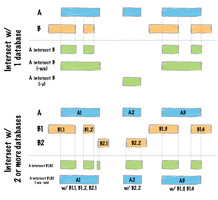
While Nanoblot allows for multiple target probes and antiprobes, the bedtools intersect function must be run one at a time for each intersection performed. If you look at the intersect diagram shown above, providing mulitple regions at once to the intersect function will render an effective OR intersection when we are looking for AND intersection. In order to subset the bam files appropriately, an intersect function must be run for each probe, one at a time.
The intermediate and final subsets of each sequencing bam file will be automatically generated in the current working director's ./temp folder, and one will be created if it does not already exist. Should the user wish to specify a specific output folder, the paramter tempFilePath to the subsetNanoblot command can be specified.
RT-PCR
An additional feature of NanoBlot is the ability to process reads in RT-PCR mode, which the user can specify by including a viewingWindow as an argument into the subsetNanoblot function. The viewing window is a genomic window with the same features as a probe, and for that reason, is included in the probes metadata file. As a result, if the genomic window is not included, the code will exit with a corresponding error that the viewing window was not found.
The RT-PCR subset essentially works the same way that the original subsetting function works, except it takes into account the inclusion and trimming of flanking regions. Reads that overlap with BOTH specified ends of the viewing window are filtered, and then sequences outside the specified ends will be trimmed until they only include within the specified ends. This is based off of how wet-bench RT-PCR reactions are performed, where the flanking sites represent extension primers that amplify a certain region of interest. First, we filter the subsetted bam files to only reads that include both the start and the end of the viewing window, as primers in a wet bench RT-pCR reaction would not amplify sequences where the flanking sites are not present. We use a bedtools intersect start and end window with a BUFFER_SIZE variable of 5 nucleotides to allow for indels at the flanking regions. After selecting for reads that include the start and end sites, we then perform a hard genomic cut that only includes the regions inside the genomic window. To do this, we use the function ampliconclip from the samtools package to clip the end of read alignments if they intersect with regions defined in a BED file. [^6]
Since ampliconclip will clip reads that overlap with the BED files, we will use the viewing window and find the complement BED entries to intersect, keeping effectively the reads that are only found within the viewing window. The options we use for ampliconclip include --hard-clip to ensure that the read width does not calculate clipped bases and --both-ends to ensure that both the 5' and the 3' ends where the regions match are cut. This genomic window is irrespective of strandedness since the reads are effectively cDNA at this point.
[^6]: Whitwham, Andrew, and Rob Davies. “Samtools Ampliconclip.” Samtools-Ampliconclip(1) Manual Page, Sanger Institute , https://www.htslib.org/doc/samtools-ampliconclip.html
An example of an input BED file for ampliconclip is as follows. Let's say our viewing window of interest is this BED file, which is the entire RPL18A gene of the Saccharomyces cerevisiae.

The viewing window line into the probes metadata file will look like this.
chrXV 93395 94402 RPL18A_vw . -We then create a temporary BED file that represents the complement genomic positions of that viewing window, which this ampliconclip will hard clip all reads that intersect this region, effectively, keeping reads that only are contained within the viewing window. The max length found in the second row represents the maximum genome size of any organism, which is found in the Japanese flower, Paris japonica, with 149 billion base pairs.
chrXV 0 93395
chrXV 94402 149000000000
Here is an example of what the result of ampliconclip will look like in IGV. It subsets all reads that overlap with the start and end of the RPL18A gene, and then trims excess nucleotides for each read that lie outside that gene window.

RACE: Rapid Amplification of CDNA Ends
Alongside the RT-PCR subsetting, there is an added 3' RACE (Rapid Amplification of CDNA Ends) option with the RACE = TRUE argument. It utilizes the same viewingWindow argument input to specify the genomic window of the RACE experiment. The only difference between RACE and RT-PCR is that whereas RT-PCR checks for inclusive ends on BOTH sides of the viewing window, RACE only checks for inclusive ends on ONE side of the viewing window, the 5' end of the specified window. Conceptually, this makes sense as the RACE protocol is used to determine regions of unknown sequences. For example, a 3' RACE experiment to determine unknown 3' mRNA sequences that lie between the exon and the poly(A) tail uses a gene-specific primer that anneals to a region of known exon sequences and an adapter primer that targets the poly(A) tail. [^7] For more information on usage, read 3' RACE protocols to see what you need. Reference manuscript for example usage.
[^7]: “3´ RACE System for Rapid Amplification of CDNA Ends.” Thermo Fisher Scientific - US, https://www.thermofisher.com/us/en/home/references/protocols/nucleic-acid-amplification-and-expression-profiling/cdna-protocol/3-race-system-for-rapid-amplification-of-cdna-ends.html.
Checking Sample Integrity
An additional method we provide is for users to check a psuedo measure of their sample integrity based off of long-read sequencing data alone. This serves as a proxy to a measure like a RIN score analysis. The function checkIntegrity takes two arguments, one which is a GRanges object from the Genomic Ranges class which contains all the expected full length features, and a BamFileList object from the Rsamtools package which contains all the original non subsetted bam files.
The integrity function then goes through each individual feature in the GeneTargets argument and calculates the percentage of full length reads over total reads that map to that given feature. For a short diagram of this overlap, please reference the paper. The function then outputs a cumulative distribitution plot that visualizes each sample's overall percetange of intact full length reads. A sample graph of this output is pictured down below.

R Plotting
Because NanoBlot deals with discrete read representations instead of continuous count numbers, the best way to visually represent the normalization is to duplicate the existing number of reads by a certain number that we call the duplication factor. This number is first calculated by taking the inverse of the size factor, since the size factor is divided during DESeq2’s count normalization, and then multiplying the inversed number by 10 and rounding to the nearest digit to account for minimal data loss. Although this duplication factor would scale each sample respectively to their normalized counts, certain samples that inherently have lower reads than others would be visually hard to see. We then assigned an arbitrary DUPLICATION_CONSTANT a value of 2000 in order to scale all samples up or down respectively to ensure equal plotting exposure. This is essentially like automatically determining the exposure for northern blots. The duplication factor from the previous step is then multiplied by taking the DUPLICATION_CONSTANT divided by the max number of reads across all samples plotted and rounded to the nearest integer. The plotting script then takes each sample’s reads and upscales it n times according to the duplication factor.